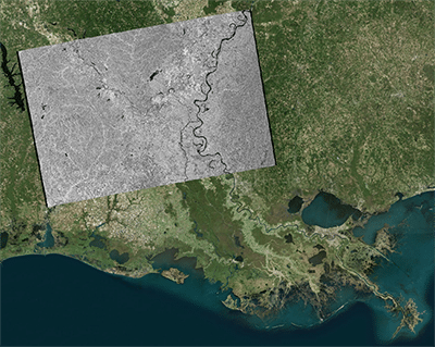
This Sentinel-1 image capturing the Mississippi River has been processed into a GIS-compatible format and imported for ease of use. Credit: Copernicus Sentinel data 2017, processed by ESA.
Adapted from coursework developed by Franz J Meyer, Ph.D., Chief Scientist, Alaska Satellite Facility and UCLA’s Technology Sandbox
● Easier
Background
Sentinel-1 Ground-Range Detected (GRD) Synthetic Aperture Radar (SAR) products are available for download from ASF’s Vertex data portal. These Level-1 GRD products are georeferenced to geographic coordinates using the Earth ellipsoid WGS84, but are still in SAR geometry.
By following this data recipe, users will learn how to geocode Sentinel-1 GRD products using the Geospatial Data Abstraction Library (GDAL) raster utilities, specifically the gdalwarp tool. GDAL is open-source, free, broadly supported, frequently updated, and can run on almost any operating system. GDAL runs on the command line, and installation is only marginally more difficult than a typical commercial application.
Why Geocode?
Once extracted from their zip file, GRD products downloaded from Vertex can be viewed directly in most GIS environments without any additional steps. The georeferenced TIFF files include the information necessary to allow most GIS software platforms to project the data layers on the fly to match the other layers in your GIS, so you can easily visualize the data without additional effort.
If you are visualizing the images outside of a GIS platform, however, the images may appear reversed or rotated. To display the images as you would expect to see them, the image must be transformed from its SAR geometry into a map projection. When working with SAR data, this process is called “Geocoding.”
Geocoding the imagery will ensure not only that the image displays at the correct location on the Earth’s surface in any given application, but that the image will also display as expected when it is viewed outside of a spatially-enabled framework (i.e. north is up, features are not stretched or reversed in unexpected ways).
Even when working within a GIS, if you want to go beyond simply visualizing the data and perform analysis or geoprocessing functions using the GRD granule, it should be geocoded to a map projection first. You may use GDAL to perform this task and then work with the geocoded products within your GIS environment, but many GIS platforms have built-in tools to accomplish this same task. If you would prefer to work directly within ArcGIS, you can use the Project Raster tool. QGIS users can use the Warp (Reproject) Projections tool in the Raster menu to run a gdalwarp command from the QGIS GUI. For more guidance on using these tools, refer to ASF’s Data Recipes for geocoding products within each of these GIS platforms.
Note that using different geocoding techniques/options may result in slight differences in the output products. While one output is not necessarily “better” than another, it is a good idea to be consistent when generating geocoded products for use in the same project, especially if you are looking at imagery from one location through time.
Why Use GDAL?
For users processing large amounts of data, or those who prefer to work outside of a GIS environment, GDAL is a logical choice. In addition, the ability to call GDAL commands from other scripting languages, such as Python, allows for easy iteration through geoprocessing tasks, or integration of geoprocessing steps into complex scripted workflows. In many cases, geoprocessing with GDAL is much faster than running a comparable tool in ArcGIS, but ultimately the best approach for any given workflow will depend on the specific goals and preferences of the user.
Geocoding is NOT Terrain Correction
It is important to understand that this geocoding process does not involve terrain correction. To match the imagery to actual features on the earth and correct for distortions caused by the side-looking geometry of SAR data, you must perform Radiometric Terrain Correction (RTC) instead. This will be particularly important in areas of high topographic variation. Refer to ASF’s Data Recipes on Radiometric Terrain Correction, or contact ASF to learn about other resources for RTC processing.
Prerequisites
Materials List:
- Windows 10, Mac OS X, or Linux
- GDAL — Geospatial Data Abstraction Library (version 2.2)
- Detailed download and installation instructions are in the How to Install GDAL section.
- Python 2.7 or higher
- Linux and Mac machines already have Python installed
- Windows users will need to download and install Python
- See the How to Install GDAL section for detailed download and installation instructions
- Users with ArcGIS Desktop software installed will already have Python 2.7 installed
- Earthdata login credentials
- If you do not already have an Earthdata account, visit the Earthdata website to register for this free service
- Download Sentinel-1 GRD data using Vertex
- You may use this Sample Granule
- When downloading from Vertex, you must either already be logged in to Earthdata, or you will be prompted to enter your Earthdata Login username and password before the download will begin.
How to Install GDAL
The GDAL project does not produce regular downloadable binaries (executables) for each release — the available version of GDAL will vary between operating systems.
If you already have GDAL installed, skip to the Geocoding Steps section.
Installing on Mac OS X
The easiest approach to downloading GDAL for Mac is to download GDAL 2.2 Complete from the KyngChaos website.
- Download the disk image
- Open the downloaded file (GDAL_Complete-2.2.dmg)
- Double-click on the Install GDAL Complete.pkg file
- You will be warned that the file is from an unknown developer. Open System Preferences, click on Security & Privacy, then click Open Anyway.
- When you are installing GDAL 2.2 with Python 2.7, a message will be displayed stating that Python 3.6 is required. For this tutorial, you can ignore the message.
- Follow the prompts to install
- Copy and paste the following line into a Terminal window:
echo ‘PATH=/Library/Frameworks/GDAL.framework/Programs:$PATH’ >>~/.bash_profile
This will allow you to run the GDAL commands without specifying a path.
- Copy and paste the following into the Terminal window:
source ~/.bash_profile
- Test your installation by typing or pasting the following command in the Terminal:
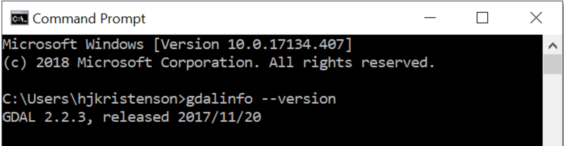
gdalinfo --version
A correct installation will output the version number followed by a release date (i.e. GDAL 2.2.3, released 2017/11/20)
Now that you have GDAL installed, you can skip forward to the Geocoding Steps section.
Installing on Linux
The method of installation will depend on your flavor of Linux. On Ubuntu, simply install the GDAL package via the Command Terminal.
To get the latest GDAL version, add the PPA to your sources, and then install the gdal-bin package. At the Terminal prompt type or paste these commands:
sudo add-apt-repository ppa:ubuntugis/ppa sudo
apt-get update
sudo apt-get install gdal-bin
To test your installation:
- Type or paste the following command in the Terminal:
gdalinfo --version
A correct installation will output the version number followed by a release date (i.e. GDAL 2.1.3, released 2017/20/01)
Now that you have GDAL installed, you may skip forward to the Geocoding Steps section.
Installing on Windows 10
Option 1: OSGeo4W Shell
The standard (standalone) installation of QGIS includes an installation of the OSGeo4W Shell. This shell has the basic appearance of the Windows Command Prompt but already has established paths to the installations of Python and GDAL that come with the QGIS installation. If you already have QGIS installed, or wouldn’t mind having QGIS installed, this is a very easy way to access GDAL.
To locate the shell, type OSGeo into the Windows Search bar. If OSGeo4W has been installed, it will appear in the list as OSGeo4W Shell (Desktop App).
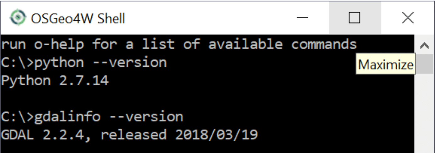
To check the QGIS versions of python and gdal, open the shell and use the commands shown in the image to the right.
Option 2: Direction Installation for Windows
If you want a flexible installation of GDAL that allows you to establish paths between GDAL and other programs or scripting GUIs, you may wish to install GDAL directly. This option has a much more involved installation process, and if you just want to give GDAL a try, you may be better served by Option 1: OSGeo4W Shell.
Install Python
Python is necessary for GDAL. If you already have an installation of Python, you may skip to Step 4 below.
- Download the latest 2.7.x version of Python (rather than the 3.x Python version)
- Install Python with the default options and directories
- After installation, open Python — IDLE (Python GUI) from the Program list
- If you can’t find IDLE, enter python into the Windows search bar, and select IDLE from the results.
- Take note of the version of Python you are running. The Python Shell window displays this information, as highlighted in the image below:
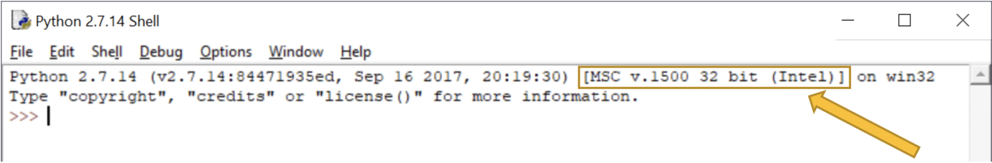
Note: For the remainder of this tutorial, we will reference the Python version as the MSC v.1500 32-bit illustrated above. If your version is different, take note and substitute that version number as appropriate in the instructions.
If you have installed the 64-bit version of Python, remove the (x86) from the paths listed in the rest of this tutorial.
Install GDAL
- Go to the GISInternals websites and find the appropriate GDAL binary.
- You may need to click on the Older Releases link in the Downloads section of the sidebar unless you have the most recent version of Python installed.
- Scroll down the Older Releases list if necessary to the newest version of GDAL available for your Python release (at the time this tutorial was written, version 2.2.3 was the most recent version available for release 1500)
- Go to the GISInternals websites and find the appropriate GDAL binary.
- Click on the appropriate release. It must match your Python version (i.e. 1500) as well as your Python architecture (win32 for 32-bit installations, x64 for 64-bit installations). Note that this is the Python installation architecture, not the architecture of your computer; you may have a 32-bit Python version installed on a 64-bit machine.
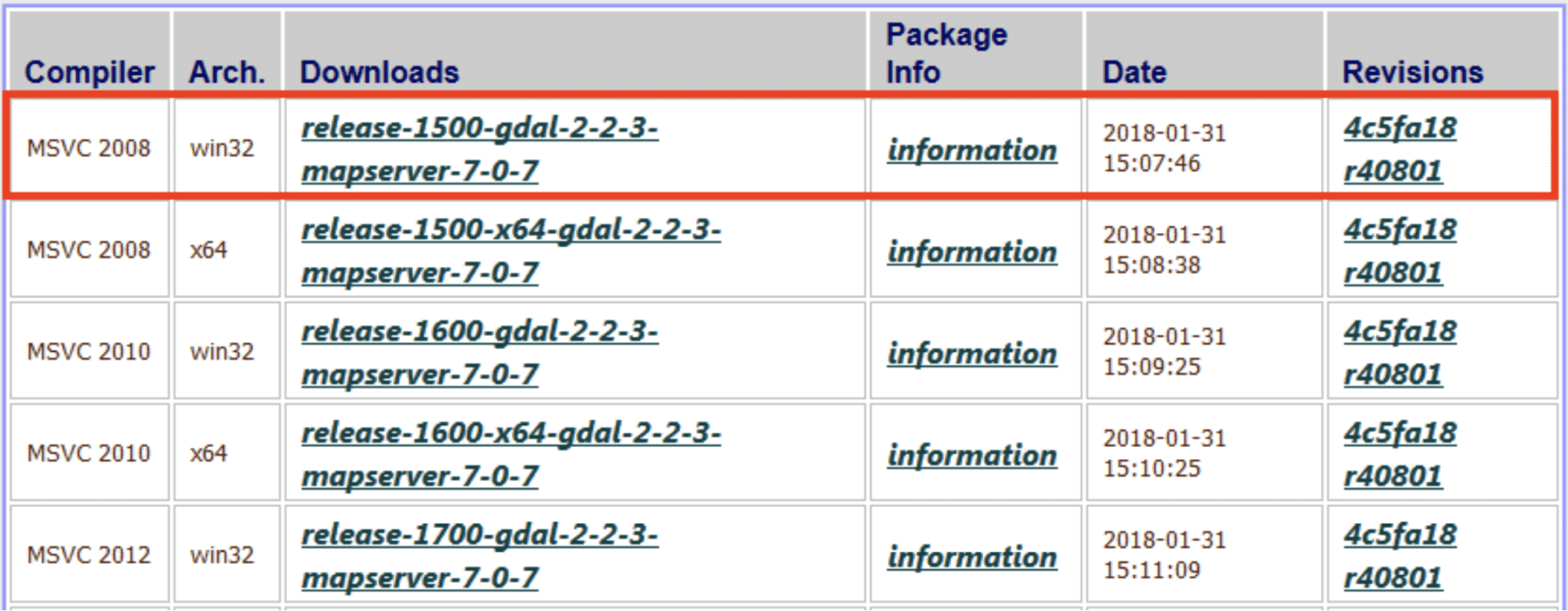
Note: For this tutorial, we are using the 32-bit MSC v.1500 version of Python; the picture below illustrates how to match the version with your own Python version. The release number (i.e. 1500) should match the MSC number for your installation.
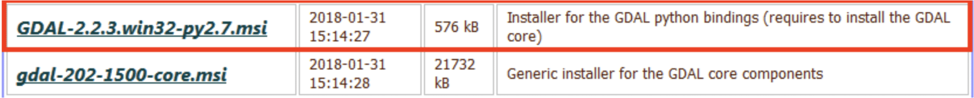
- Clicking the appropriate release link will take you to a list of binaries (installers) to download.
- Locate the “core” installer, which has most of the components for GDAL, and click the link to start the download.
- After downloading your version, install GDAL with standard settings.
- Return to the list of GDAL binaries and find the Python bindings for your version of Python (i.e. Python 2.7, win32).
- Click the link to download the Python bindings, and install them on your computer.

Add Path Variables
We need to add some system variables to tell the Windows system where the GDAL installations are located.
- Open a File Explorer window
- Right-click on This PC (or My Computer) and select Properties
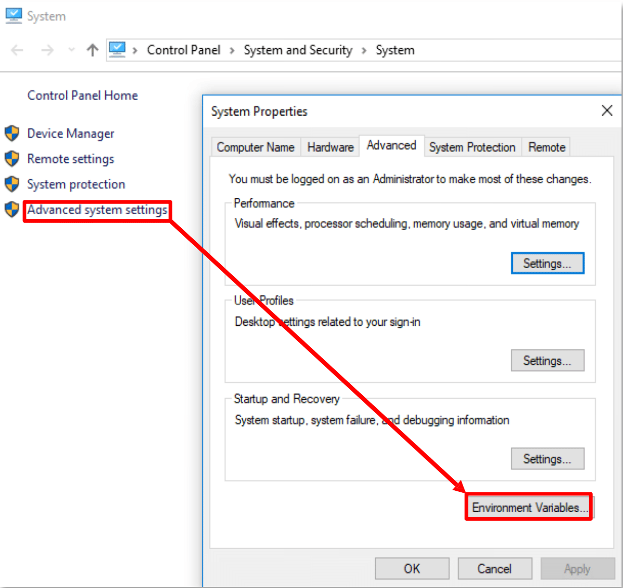
- Click on Advanced System Settings.
- Click the Environment Variables button in the System Properties window
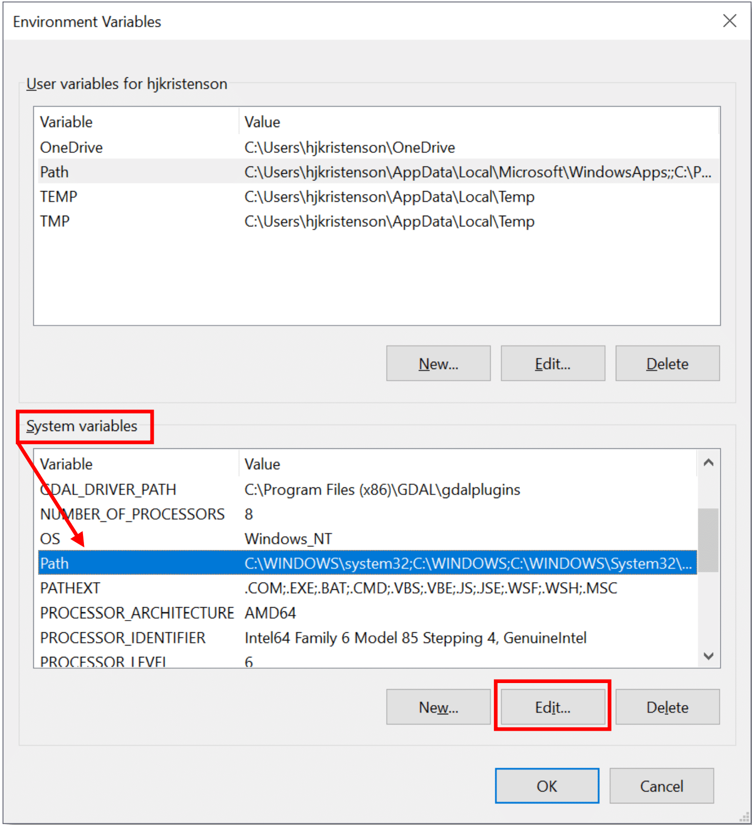
- Under the System Variables pane, click on the Path variable to highlight it.
- Click the Edit button beneath the System Variables Window.
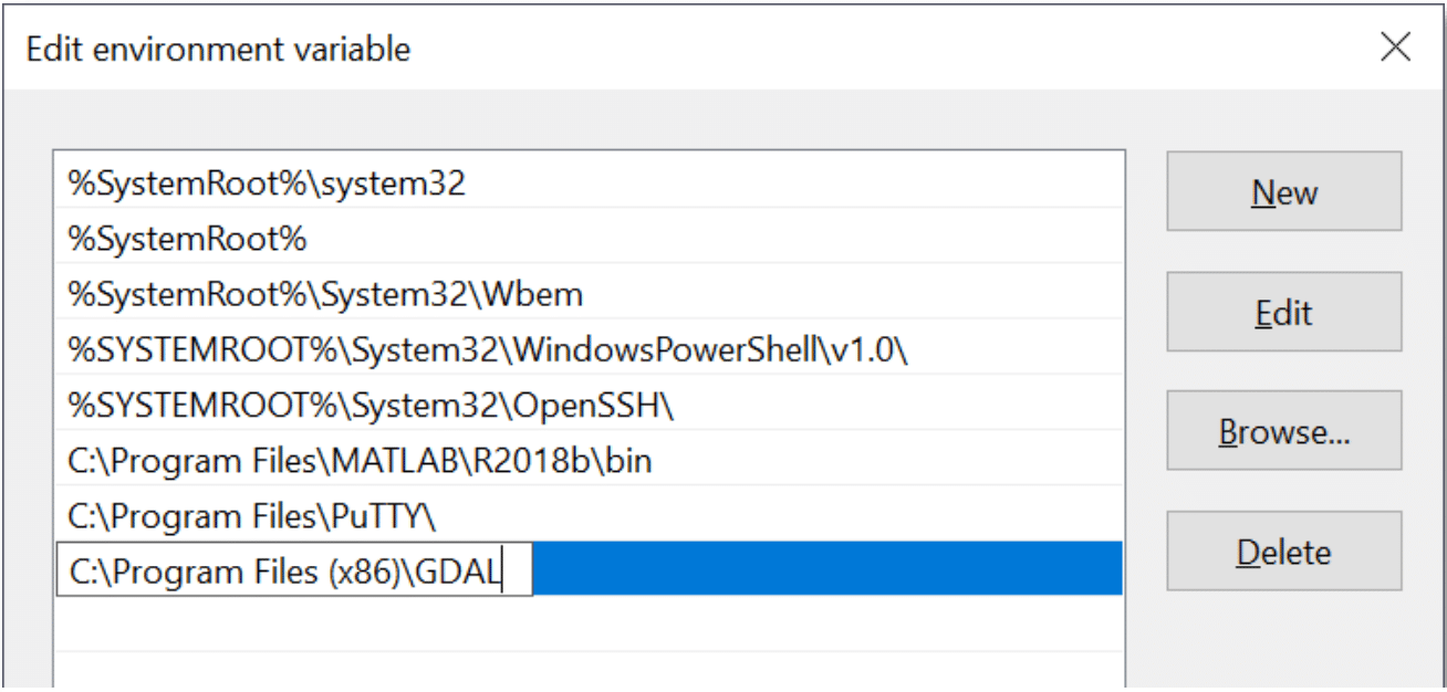
- Click the New button (or double-click in the next empty line at the bottom of the list), and enter the following path: C:\Program Files (x86)\GDAL
- For a 64-bit GDAL installation, you must remove the (x86) from the path.
- Click OK to close the Edit Environment Variable window
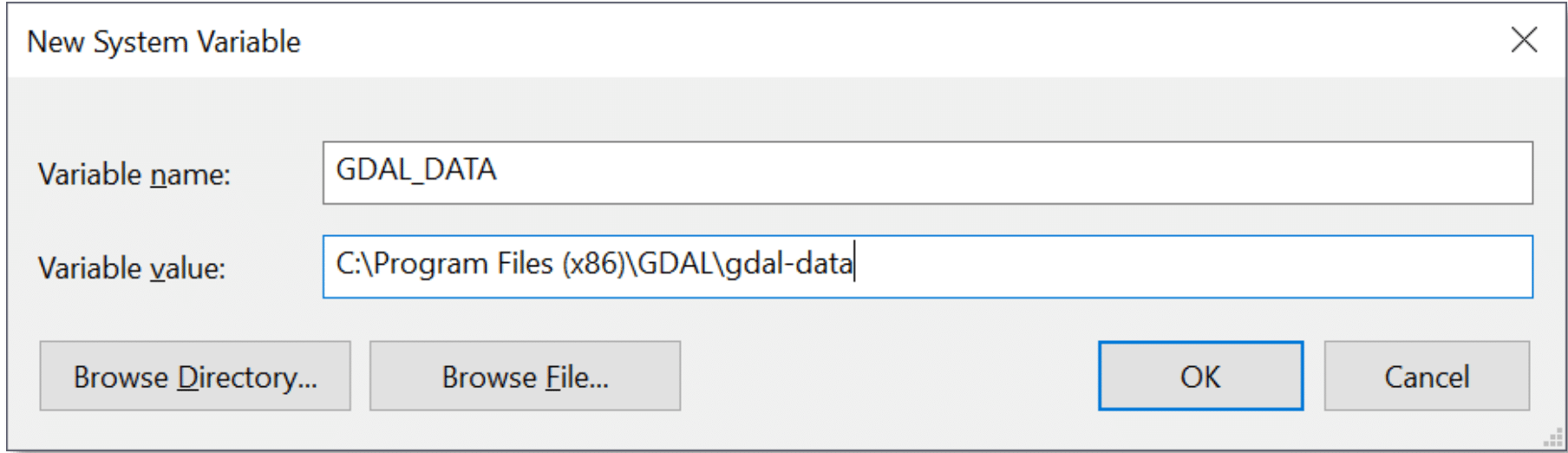
- Beneath the same System Variables pane, click the New button (next to Edit)
- Add the following in the dialog box:
- Variable name: GDAL_DATA
- Variable value: C:\Program Files (x86)\GDAL\gdal-data
- Click OK to return to the Environment Variables, and click the New button again
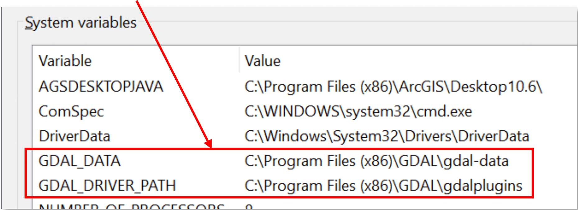
- Create another new System Variable by adding the following in the dialog box:
- Variable name: GDAL_DRIVER_PATH
- Variable name: C:\Program Files (x86)\GDAL\gdalplugins
- Click OK to return to the Environment Variables, where you should now see your new paths listed
- Click OK to close the Environment Variables window
- Click OK to close the System Properties window
- Test your installation:
- Open Command Prompt (type cmd in the Windows search bar to find the application), type in the following command and press enter:
gdalinfo --version
- A correct installation will output the version number followed by a release date (i.e. gdal 2.2.3, released 2017/11/20)
Once GDAL is successfully installed on your computer, proceed to the Geocoding Steps section.
Geocoding Steps
For this tutorial, you will use the GDAL raster utilities gdalwarp and optionally gdal_translate.
Extract the .tiff file with the Data of Interest
Within the downloaded zip file is a base directory with the name of the granule followed by a .SAFE extension. This SAFE structure contains a number of directories and files, and the data images are saved as georeferenced .tiff files in the folder named “measurement.”
The image we are interested in for this tutorial is the co-polarized GRD:
s1b-iw-grd-vv-20181209t004115-20181209t004140-013958-019e67-001.tiff

Note: If you are using a different granule than the sample provided, the co-pol image may be labeled hh instead of vv.
Use your preferred method to extract the desired file from the zipped folder, or see below for suggestions:
Unzipping with OS X or Linux
Using the Unix unzip utility (also works with OS X) in the command terminal, you can extract just the file you want from the downloaded zip folder (filename.zip) with a command like this:
unzip <filename.zip> */measurement/*vv*.tiff
This will extract just the VV polarized image from this zip package. If you know which file you want, this is usually much faster than extracting the whole zip file.
Unzipping with Windows 10
If you unzip the entire folder with the standard Windows 10 zip utility, there is a good chance that you will exceed the number of characters allowed in a Windows directory path. You can either save the zipped contents to a different folder, or you can just extract the single file as follows:
- Double-click the .zip file in your Downloads folder, double-click the .SAFE file, double-click the measurement folder and highlight the desired .tiff file.

- Under the Compressed Folder Tools menu (which appears when you browse into a zip file), click the Extract button and select the Extract To… option.
- Select one of the recent folders (which will start the extraction immediately), or use the Choose Location option at the bottom of the dialog box to navigate to the desired extraction location and click the Copy button to extract the file.
- The single .tiff file will be extracted from the zipped folder structure.
You may also wish to download the 7-Zip File Manager for a more flexible zip utility than the standard Windows zip utility.
Project your Product using gdalwarp (Geocoding Step)
You can use the GDAL command line utilities to project and export files. The corner coordinates for Sentinel-1 data are provided in geographic coordinate system (GCS) coordinates (latitude/longitude), but can easily be changed into another projection.
Determine the European Petroleum Survey Group (EPSG) projection code for your image location
The sample granule provided is located in Lousiana, which is UTM Zone 15N (EPSG 32615). If you know the EPSG code for your projection, that’s all you need for the spatial reference option in the gdalwarp command. If you don’t know the projection code, you can search for it in the Spatial Reference database. You may search or browse to the spatial reference you are interested in.
Note that some projections (such as UTM Zones) have different EPSG numbers for coordinates in the northern hemisphere vs. the southern hemisphere.
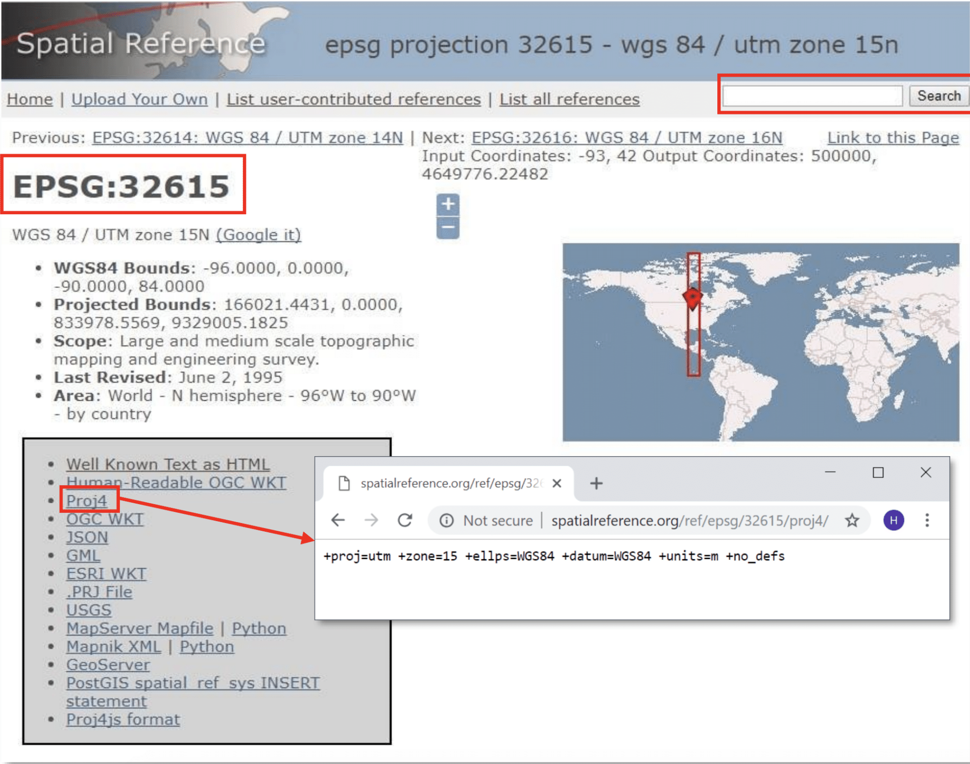
If the projection you want to use does not have an EPSG code, you can click on the Proj4 link to display a text definition of the projection. This text can be enclosed in single quotes and used in place of the EPSG code in the gdalwarp command. For some projections where EPSG codes are different depending on the hemisphere (i.e., UTM north/south), the text definition of the projection may be the same regardless of hemisphere. If the Proj4 link is empty, that particular projection is probably not yet supported by GDAL.
Open a Command Terminal or OSGeo4W Shell
- To open a Command Terminal in Windows, type “cmd” into the Windows search bar to find the Command Prompt desktop app, or navigate to it in the Windows System folder in the Programs list.
- To open the OSGeo4W Shell, type “OSGeo” into the Windows search bar to find the OSGeo4W Shell Desktop application, or navigate to it in the QGIS or OSGeo4W folder in the Program list (location will depend on the installation choices you made).
In the Command Terminal or OSGeo4W Shell, browse to the directory where you saved your extracted GRD .tiff product.
| Command | Purpose | |
|---|---|---|
| cd < directory> | Change directory | |
| cd .. | Navigates to parent directory (one folder up) | |
| Windows, OSGeo4W Shell commands: | ||
| dir | List directory contents | |
| cd | Display path of current directory | |
| x: | Change disk drive (i.e., enter G: to change from the C: drive to the G: drive) | |
| Linux, OS X commands: | ||
| ls | List directory contents | |
| pwd | Display path of the current directory | |
Use the gdalwarp command to geocode the file
The gdalwarp command consists of the following components, which will be typed together in one command in the Command Terminal, as demonstrated by the example below (color-coded here to illustrate the different components; component descriptions will follow):
gdalwarp -tps -r bilinear -tr 10 10 -srcnodata 0 -dstnodata 0 -t_srs EPSG:32615
s1a-iw-grd-vv-20170819t001029-20170819t001054-017985-01e2e8-001.tiff s1a-iw-grd-
vv-20170819t001029-20170819t001054-017985-01e2e8-001-utm.tif
-tps specifies to use the thin plate spline technique when interpolating the ground control points. This is optional, and not available when projecting images using either ArcGIS or QGIS, but you may get a slightly better image fit using this technique.
-r specifies the resampling method (default is nearest neighbor); set this to bilinear.
-tr specifies the output pixel size, in the units of the output projection; in this example, we set it to 10×10 meters (UTM coordinates are in meters).
-srcnodata (optional) sets the mask values in the input TIFF to NoData; data from Vertex may have had 0 values added to mask bad pixels, and these mask pixels will be converted to NoData values. Omit this option if you want to retain the 0-values in the mask pixels from the source image.
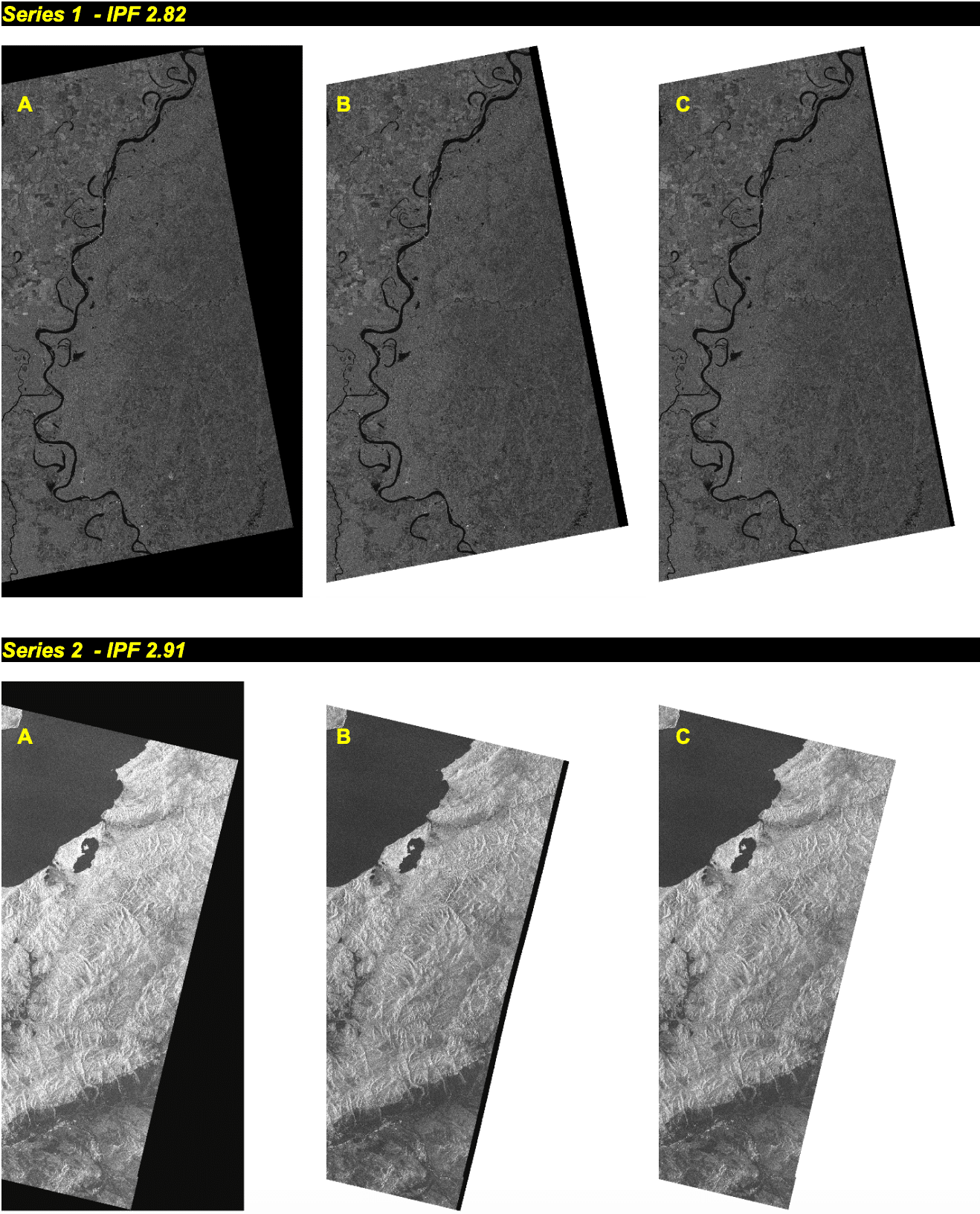
Note that ESA has applied different masks to the Level-1 products over time. While it is always okay to set the 0 values to NoData, older products will have more garbage pixels left over. Only in March 2018 (IPF 2.90) did ESA start masking all of the artifacts at the image edges with 0 values; using the srcnodata option with this newer data results in a nice, clean image free of edge artifacts. Refer to ESA documentation for more details.
-dstnodata (optional) sets the padding values generated by the gdalwarp command TIFF to NoData; if this option is not used, the output file will include 0 values around the edge of the image, which will display as black. If you prefer, you can set the padding pixels to NoData later with additional gdal command or within a GIS software program, but this option outputs data directly with transparent padding pixels.
-t_srs specifies the output projection; for this example, enter the EPSG code. To use the text definition of the projection instead, enclose the text in single quotes (i.e., -t_srs ‘+proj=utm +zone=15 +ellps=WGS84 +datum=WGS84 +units=m +no_defs’)
[input file] the name of the input file; note that this follows the options directly without any additional dashes
[output file] the name of the output file; this is the last item included in the command. If you will be using the output file in ArcGIS, you may wish to use a .tif extension rather than .tiff, which causes problems in some geoprocessing tools.
Note: the input and output filenames in this example assume that you are in the directory containing the input file and want the output file saved to the same directory. If you are NOT running the command from the same directory as the input files, you will need to type in the FULL PATH, not just the filename. Similarly, if you want the output to be saved in a directory other than the current directory you will need to type in the full directory path for the output file.
- Type the gdalwarp command with the desired options into the Command Terminal and press Enter to run the command.
- You may adjust the gdalwarp command options according to your needs and preferences, and there are many additional command options available. Refer to gdalwarp documentation.

At this point, your output has been geocoded to a map-projected GeoTIFF file that can be used in any image viewing or GIS platform or additional GDAL processing that can be applied. The gdal_translate utility allows a user to convert raster data to different formats, allowing for rescaling, resizing and resampling.
Note that the images may appear all black and you may need to adjust the color scaling in your image viewer. When viewing the images in a GIS, try setting the display to stretch to 2 standard deviations for a start and adjust as necessary.
Optional — Scale to byte
The Level-1 GRD images are quite large, and you may wish to scale the pixel values to allow for faster processing. By default, the -scale option in gdal_translate uses the min and max values of the source data as the src_min and src_max, and 0 to 255 for the output value range, but if you have a certain range of values that are of particular interest, you could set your src_min and src_max to custom values.
For example:
gdal_translate –ot Byte –scale 0 700 0 255 <infile.tif> <outfile.tif>
In this case, we are converting from long integer values to byte values. Values greater than 700 in the source data will all become 255, source values less than 0 (there shouldn’t be any in a GRD) will all become 0, and the source values between 0 and 700 will be scaled appropriately between 0 and 255.