

| Parameter | Value |
|---|---|
| Temporal Coverage | June – October 1978 |
| Spatial Coverage | Oceans, sea ice |
| Center Frequency | 1.275 GHz (L-Band) |
| Polarization | Horizontal transmit, horizontal receive (HH) |
| Spatial Resolution | 25 m azimuth x 25 m range |
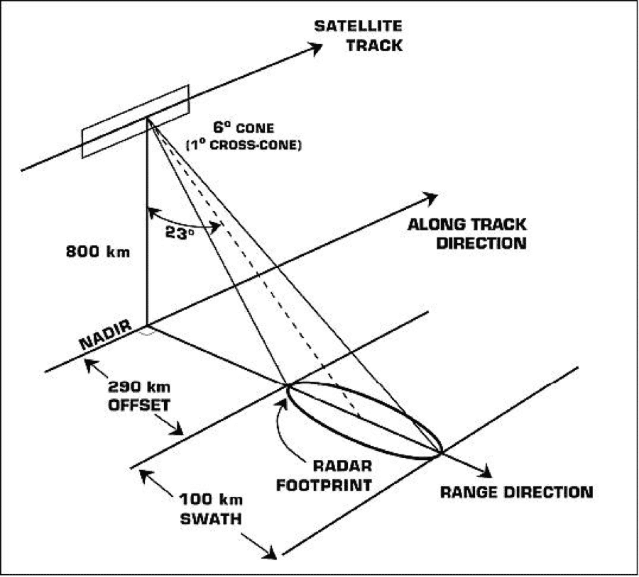
| Swath Width | 100 km |
| Off-Nadir Angle | 108° |
| File Format | Geotiff or HDF5 |
| Download Information | Data Discovery |
| Date Published | 2013 |
| System Bandwidth | 19 MHz (linear FM) |
| Satellite Altitude | 800 km |
| Pulse duration | 33.4 us |
| Antenna Dimensions | 10.74 m x 2.16 m |
| Ground incidence angle | 23°± 3° cross track |
| No. of looks | 4 |
| Data recorder bit rate (on the ground) | 110 Mbits/s (5 bits/word) |
| Radar Wavelength | 23.5 cm |
| Pulse Repetition Frequency (PRF) | 1463-1640 Hz |
| Antenna Look Angle | 20° from vertical (fixed) |
| Antenna type | 1024-element passive micro-strip based arrays antenna, linearly polarized |
| Transmitted peak power | 1 kW |
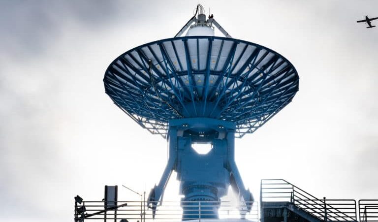
Seasat Satellite’s Synthetic Aperture Radar History
Seasat set a Landmark in Remote-Sensing History in 1978. On June 27 GMT, 1978, NASA undertook a momentous task: launching the Seasat satellite in order to demonstrate the feasibility of orbital remote sensing for ocean observation. On board was the first NASA synthetic aperture radar sensor ever deployed.
This mission supplied the decades-old data that the Alaska Satellite Facility, a NASA Distributed Active Archive Center (DAAC), has processed into a treasure trove of digital images. The new imagery enables scientists to travel back in time for research on oceans, sea ice, volcanoes, forest land cover, glaciers, and more. Before now, only a small percentage of Seasat data was processed digitally.
Although Seasat suffered a catastrophic power failure on October 10, 1978, in 106 days the satellite collected more synthetic aperture radar information about the ocean surface — its primary mission — than had been acquired in the previous 100 years of shipboard research.
Synthetic aperture radar, also known as SAR, bounces a microwave radar signal off the surface of Earth to detect physical properties. Unlike optical photo technology, SAR can see through darkness, clouds, and rain.
The scientific value of Seasat’s SAR is extensive, providing unique and unexpected views of the dynamic ocean surface and sea ice cover, as well as the vegetated, exposed, populated, and cold regions of Earth’s surface. ASF’s new suite of Seasat products are likely to be valuable in a range of scientific disciplines, particularly for studies that measure features of the planet’s surface over time. Examples include the following:
- Boreal forest land cover between 1978 and 1997 could be compared using data from Seasat and the Japanese Earth Resources Satellite 1 (JERS-1).
- Rates of deformation over known active faults in North America and Pacific Rim volcanoes could be studied using Seasat’s seven orbit cycles of 3-day repeat data.
- Glacial change observations based on data acquired in 1978 over Norway and Alaska could establish a much older baseline than is currently available from other sensors.
In addition to SAR, Seasat satellite instruments included a radar altimeter, a scatterometer, a scanning multichannel microwave radiometer, and a visible/infrared radiometer.
Seasat Image Examples
| Image Examples |
|---|
 |
| Grays Harbor and Willapa Bay in Washington State. ASF Granule SS_00638_STD_F0928 captured August 10, 1978. © NASA. |
 |
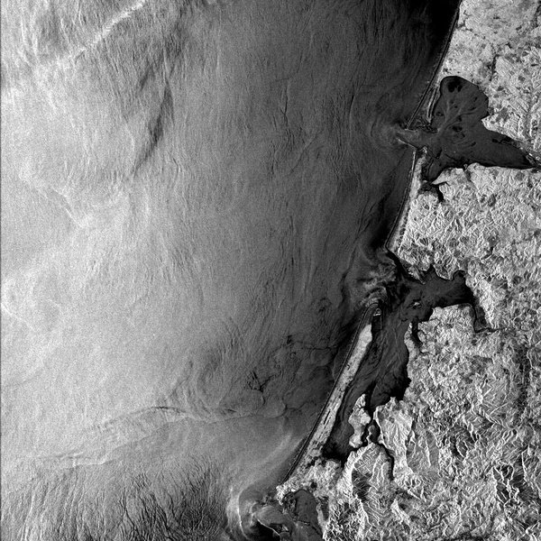
| Mouth of the Columbia River and the Oregon coastline. ASF Granule SS_00638_STD_F0914 captured August 10, 1978. © NASA |
 |
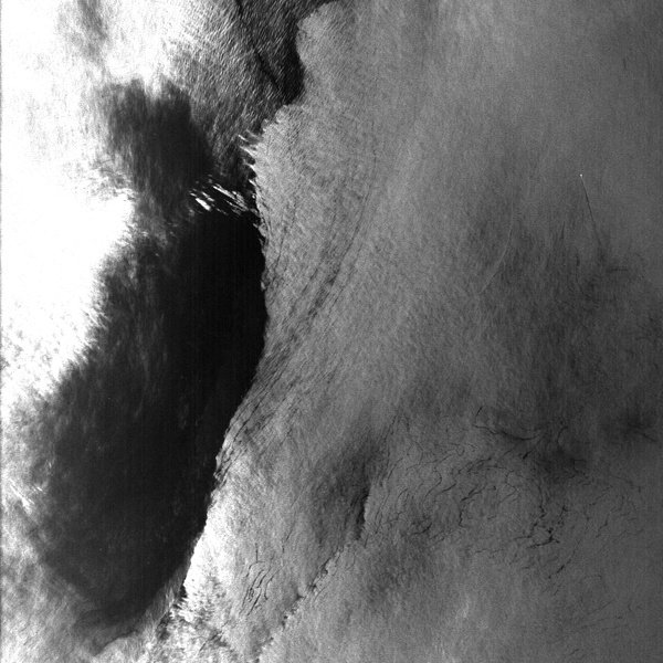
| The North Sea off the coast of England. View full image to see two boats and their wakes in the top half of the image. ASF Granule SS_00785_STD_F2511 captured August 20, 1978. © NASA. |
 |
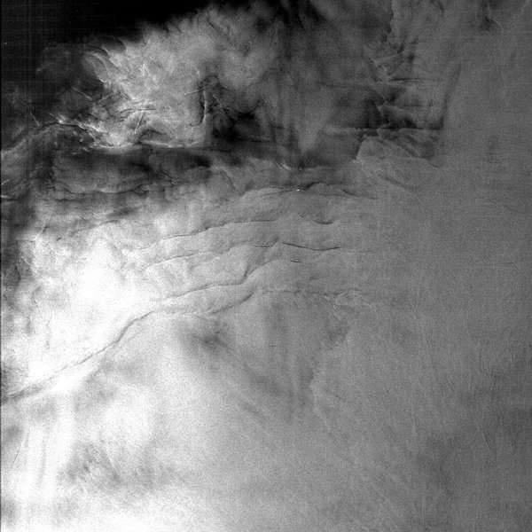
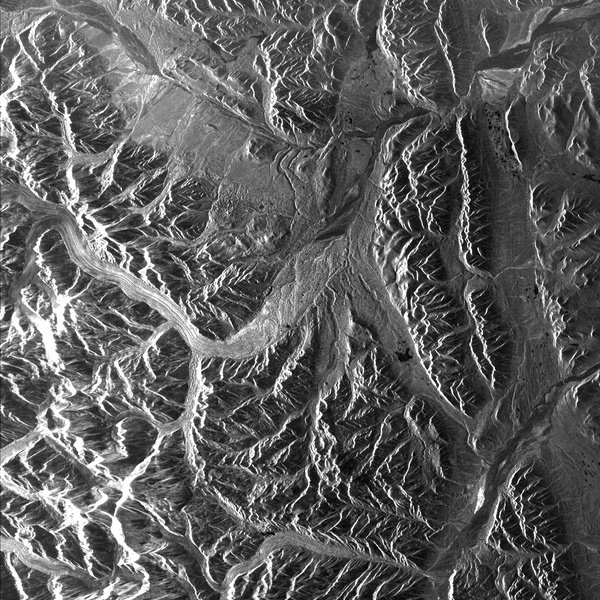
| A scene from northeast Russia. ASF granule SS_00492_STD_F2241 collected August 20, 1978. © NASA. |
 |
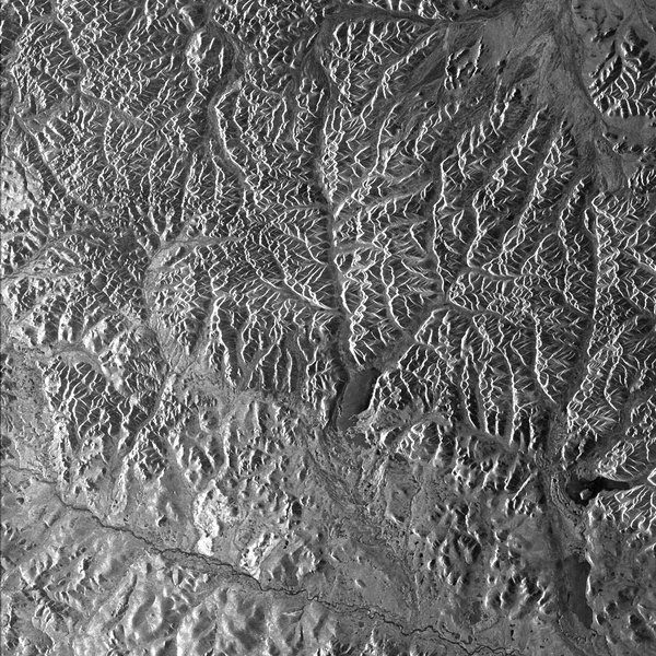
| A scene from Teepee Park, Yukon, Canada. ASF granule SS_00351_STD_F1224 collected July 21, 1978. © NASA. |
 |
| Isla Cedros, Baja California. ASF Granule SS_00351_STD_F0556 collected July 21, 1978. © NASA. |
 |
| Uncle Sam Bank, Pacific Ocean, Baja California. View full image to see a boat as a small white dot in the upper right quadrant. ASF Granule SS_00351_STD_F0499 collected July 21, 1978. © NASA. |
User Guide/Technical Information
Instrument and Launch
Seasat was launched aboard the Atlas-Agena on June 26, 1978, from Vandenberg Air Force Base in California. The Seasat spacecraft itself weighed 2,300 kilograms.
The launch sequence of Seasat went smoothly. The satellite, called Seasat-1 in orbit, had established communications and deployed its solar panels as well as sensor antennas during the second and third orbits. It then extended its synthetic aperture radar antenna.
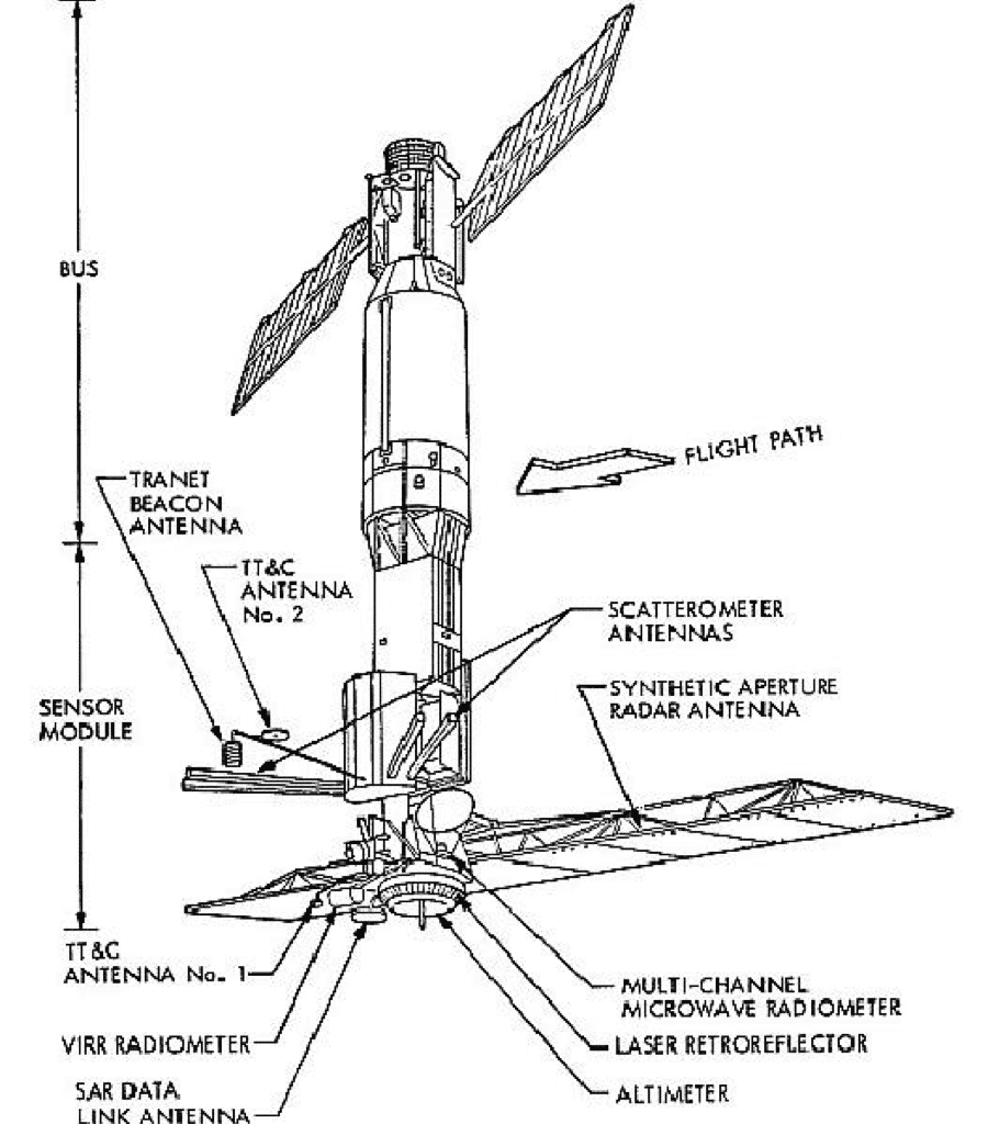
Sensors
Seasat’s five onboard sensors were individually managed by the following centers:
- Radar altimeter: Wallops Flight Center
- Scanning Multichannel Microwave Radiometer (SMMR) and Synthetic Aperture Radar (SAR): Jet Propulsion Laboratory
- Seasat-A Scatterometer System (SASS): Langley Research Center
- Visible and Infrared Radiometer (VIRR): Goddard Space Flight Center
- Synthetic Aperture Radar
The SAR instrument onboard Seasat weighed 147 kilograms and consumed approximately 216 watts of power (1000 watts peak). As such, the SAR sensor could only be operated for 10 minutes per orbit, resulting in a total of approximately 42 hours of SAR data being recorded over the 106-day lifetime of Seasat.
The planar SAR antenna array consisted of eight, 1.3 m x 2.16 m, rigid and structurally identical fiberglass honeycomb panels. The panels were hinged together in series but were individually supported by a deployable tripod substructure that governed the deployment of the truss and provided the interface of the antenna structure with the spacecraft. The Seasat SAR sensor is regarded as the first imaging SAR system used in Earth orbit.
Originally, Seasat SAR data were optically processed into survey data products available on 70 mm film. Approximately 10 percent of the total Seasat SAR dataset was digitally processed by the Jet Propulsion Laboratory (JPL) from 1978 and 1982. Those digitally processed products contained complete 100-km-wide swaths of data.
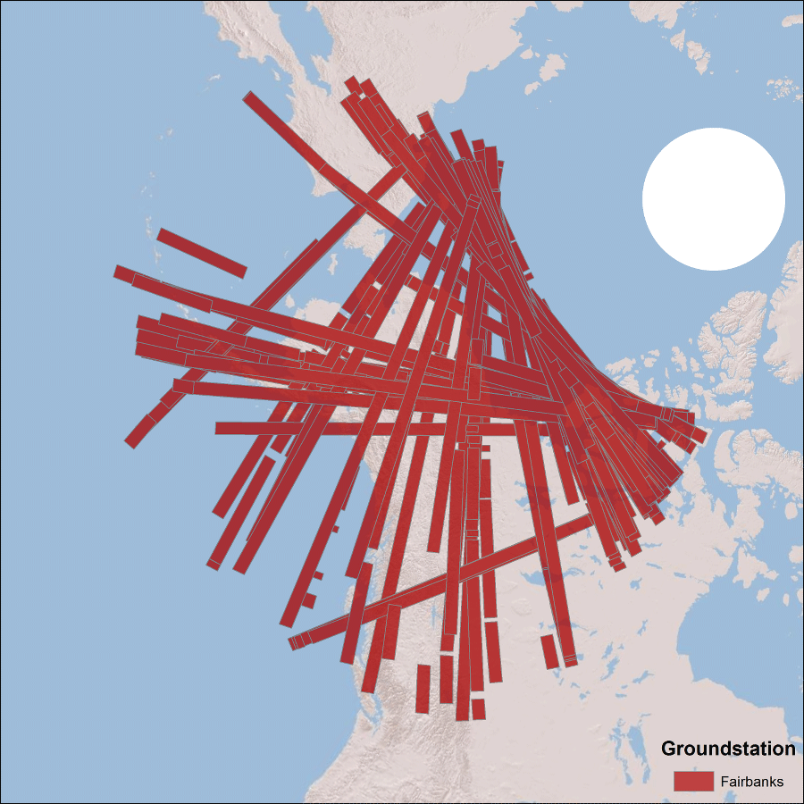
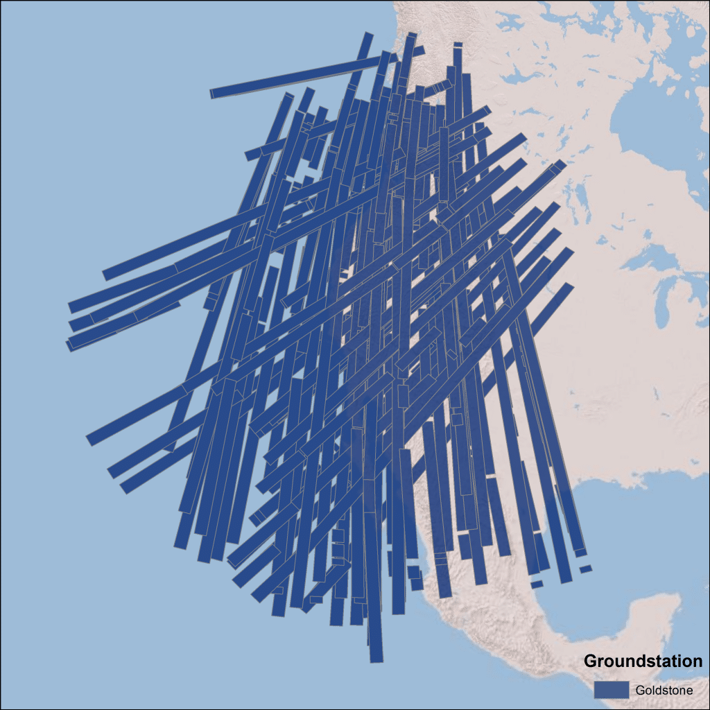
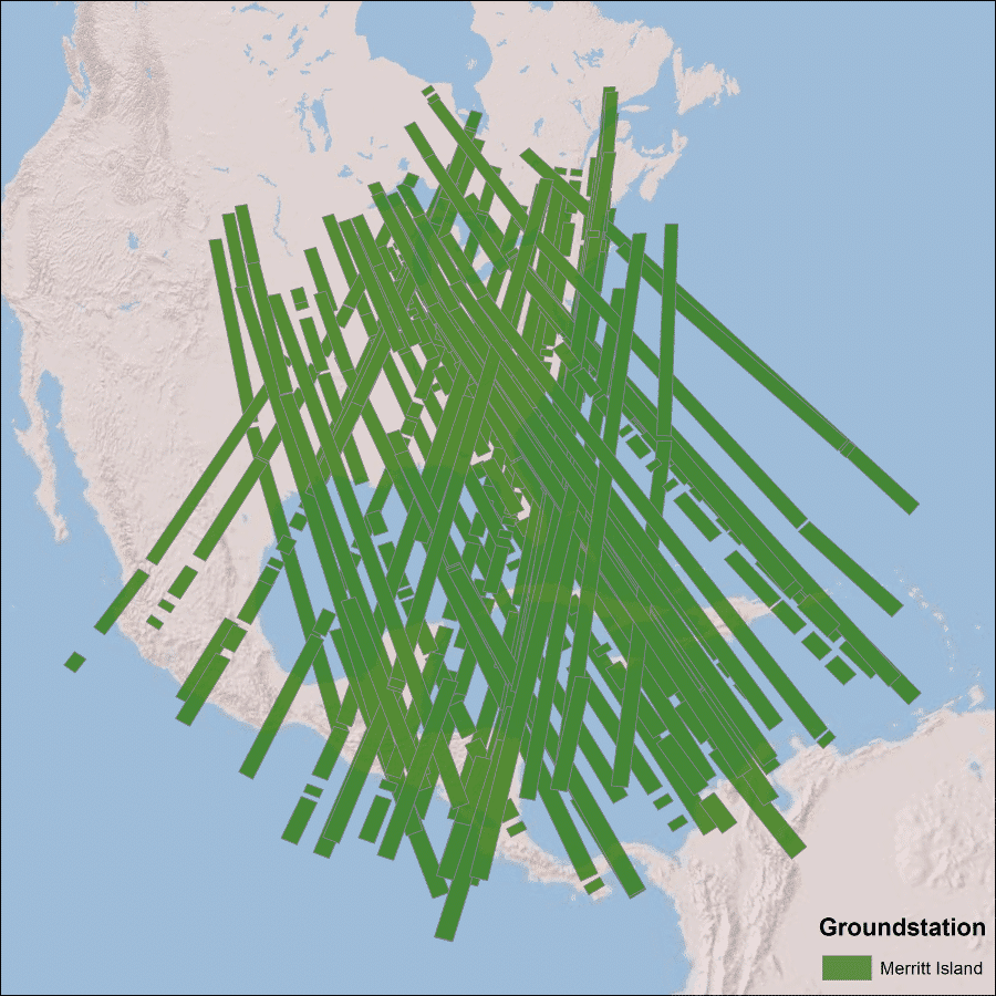
Seasat did not have an onboard recording capability for data. Therefore, the received SAR echoes were downlinked in real-time to five ground receiving stations: Goldstone, California; Fairbanks, Alaska; Merritt Island, Florida; Shoe Cove, Newfoundland; and Oakhanger, United Kingdom. The SAR data were transmitted from the satellite to the ground stations in a 20 MHz analog data stream.
Technical Specifications
| Seasat SAR Sensor Parameters | Value |
|---|---|
| Polarization | HH |
| Look direction | Right |
| Footprint | 100 km X 15 km |
| Image frame size | 100 km X 100 km |
| Image Resolution | 25 m |
| Number of looks | 4 |
| Bandwidth | 19 MHz |
| Slant range resolution | 6.6 m |
| Ground range resolution | 17-23 m (based on incidence angle) |
| Frequency | 1275 MHz – L-Band |
| Radar Wavelength | 23.5 cm |
| Pulse duration | 33.8 microseconds |
| Sampling Rate | 45.53 MHz |
| Sampling Time | 21.97 nS |
| Sampling Window Duration | 288 microseconds |
| Incidence Angle | 23 +/- 3 degrees |
| Pulse Repetition Frequency | 1647 Hz |
| Data sample size | 5-bits |
Viewing Geometry
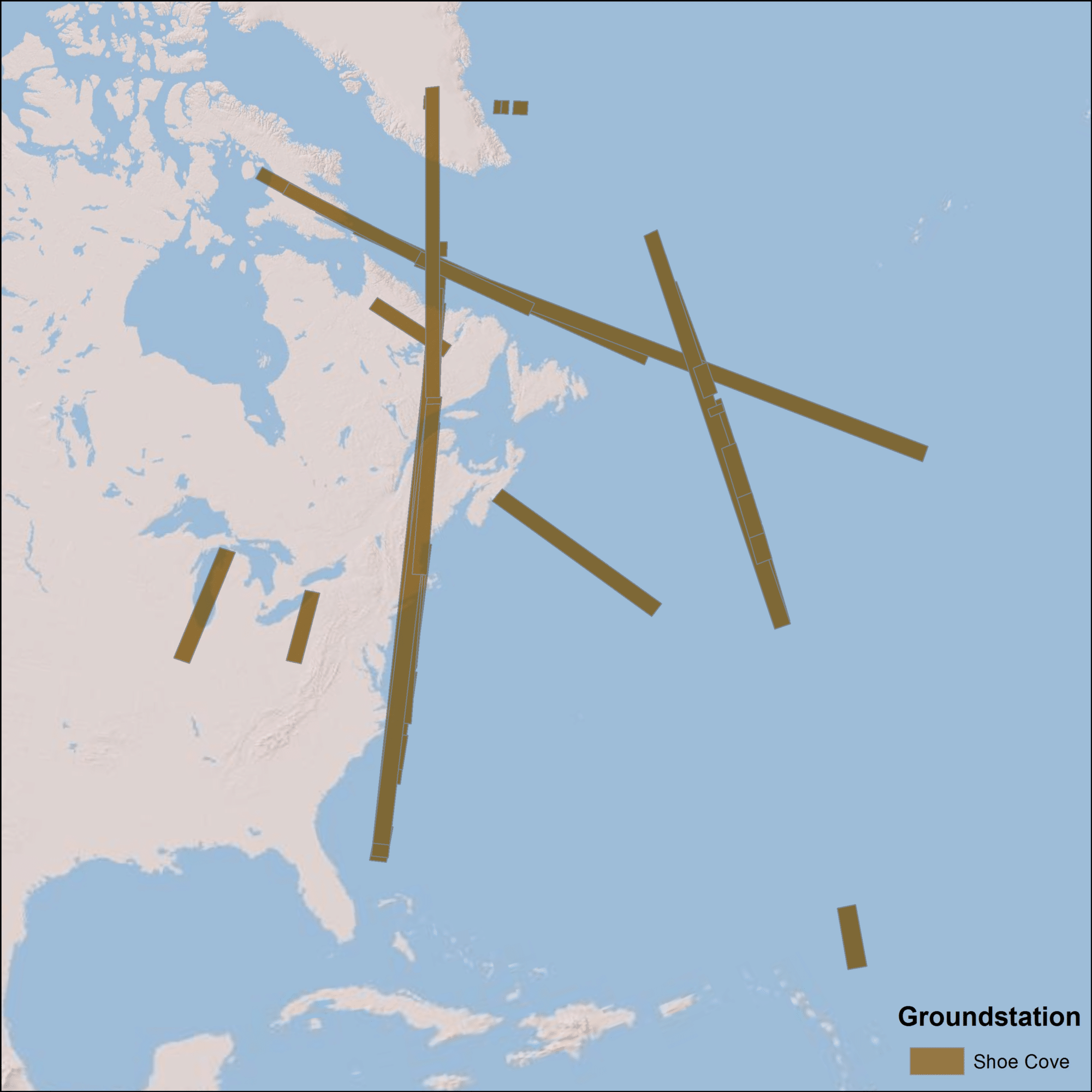
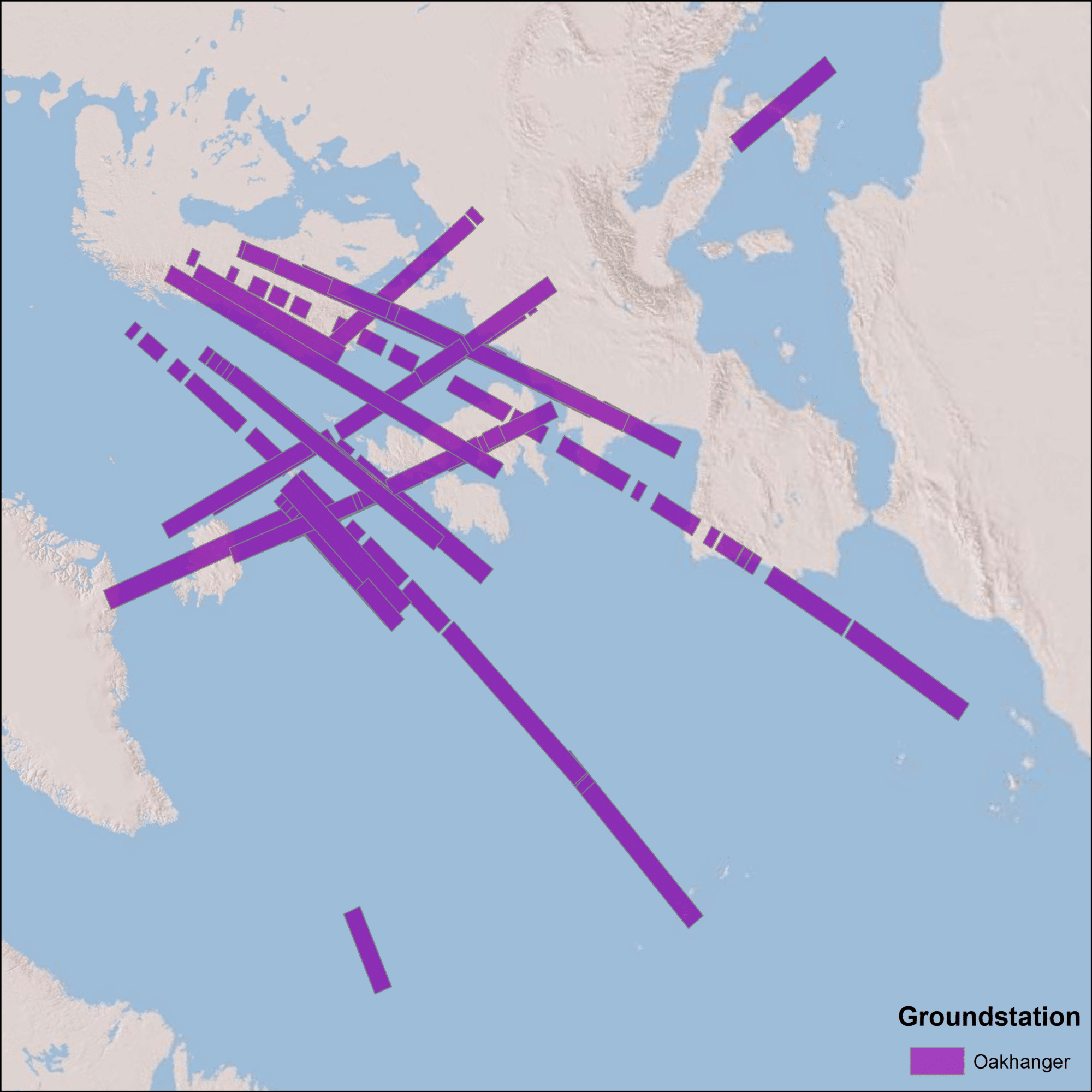
Seasat – Swath Coverage Maps
The Seasat satellite was designed to cover areas up to 75° north latitude. Seasat data was acquired by five ground stations in the Northern Hemisphere. The coverage map above displays the location of Seasat products that have been processed by the ASF DAAC. Note: All Seasat frames undergo visual inspection, so frames displayed in the above map may not be immediately available for search and download via Vertex.
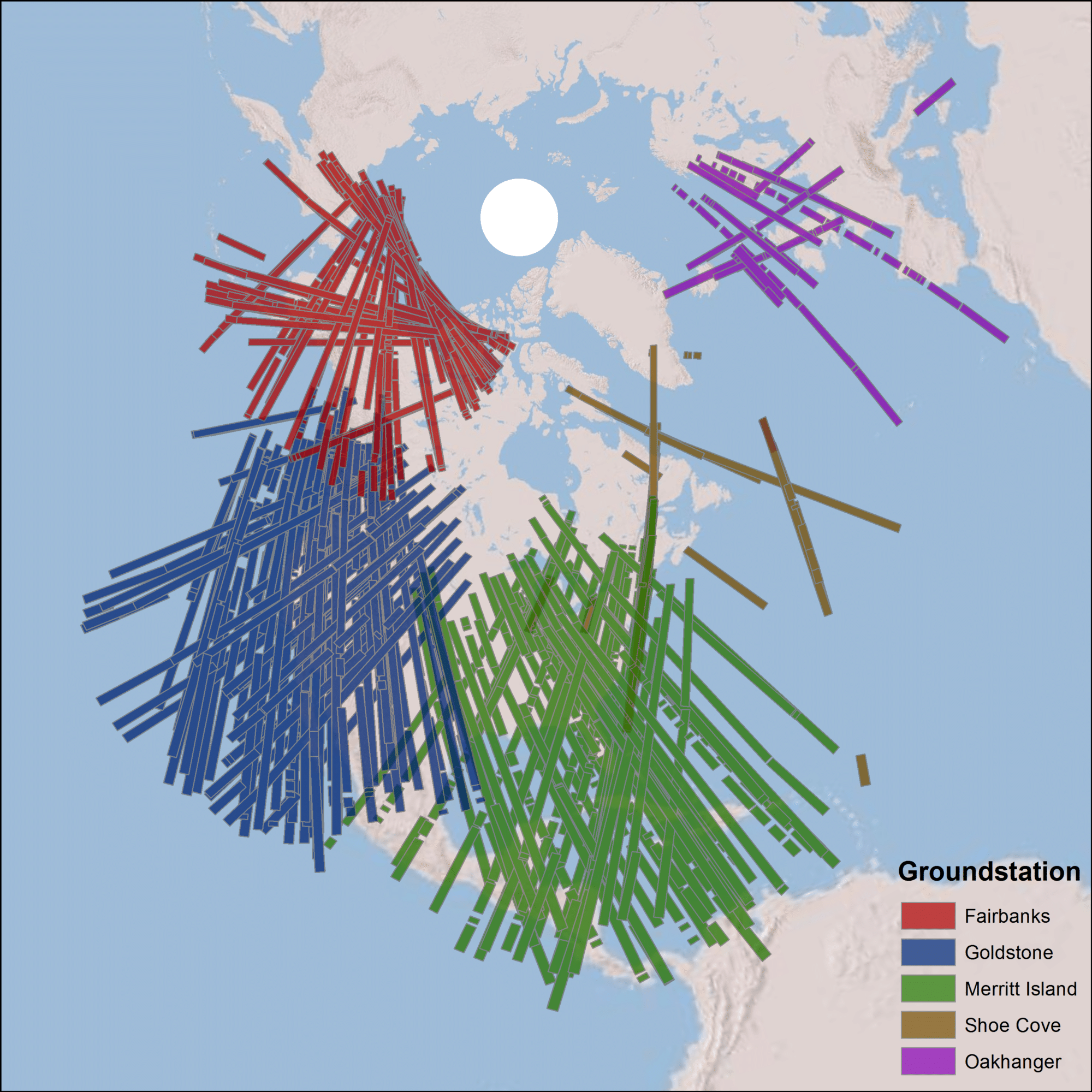
Fairbanks, Alaska
Goldstone,California
Merritt Island, Florida
Shoe Cove, Newfoundland
Oakhanger, United Kingdom
Glossary of Terms
| Term | Definition |
|---|---|
| Azimuth / Along-track | The direction the satellite is moving. SAR can be referred to in (Range, Azimuth) coordinates using either time or distance (since time and distance are interchangeable in a SAR system). |
| Azimuth Reference Function | A frequency-modulated chirp whose parameters depend on the velocity of the spacecraft, the pulse repetition frequency (PRF), and the absolute range. The chirp is Fourier transformed into Doppler space and multiplied by each column of range-migrated data in order to focus the data in azimuth, accounting for the phase shift of the target as it moves through the aperture. |
| BER | Bit Error Rate. |
| Bit | One binary digit. |
| Byte | Eight binary digits. |
| Caltones | Calibration tones. |
| Chirp | A waveform created by sweeping the frequency from low to high. |
| Cleaned File | Decoded signal file that has all currently addressed data errors corrected. |
| Datatake | One pass of the satellite over a ground station. Since the satellite was constantly imaging and sending telemetry packets, a datatake will contain a contiguous swath of radar echoes from the ground. |
| Decode | Decode (of Telemetry) is the process of unpacking telemetry packets into usable data. Generally, a telemetry packet will have three parts: |
| 1. Sync Code — Packets start with a synchronization code (sync code), this is a recognizable pattern that signals the start of a data packet. It is vital in determining the start of packets, and thus, how to interpret the rest of the information in a packet. | |
| 2. Metadata and Status — Next follows some metadata, generally containing timing information and satellite status. These are typically packed into the smallest number of bits possible. Thus, they have to be interpreted and expanded in order to gain information about the data packet that was received. | |
| 3. Payload — Finally, each telemetry packet will contain some amount of payload, i.e. actual data samples. Again, these will be packed into as few bits as possible and thus must be decoded into usable data sizes (typically, byte values). Additionally, it is common for a single payload to be so small as to not be able to contain an entire “line” of an image. Thus, in most cases, multiple payloads have to be combined to create a single imaged line. | |
| Delay to digitization | Parameterizes the time between when a satellite emits a pulse and when return echoes are recorded. Field in Seasat metadata. |
| ESA Standard Nodes | Node locations defined by ESA to tag images at a given location. For node 0 to 1800 the center latitude is (node * 0.05) degrees, while for nodes 1801 to 3600 the center latitude is 180.0 – (node * 0.05) degrees. |
| Fill flag | Fill Flag should be 1 when no valid SAR data is sent, 0 if payload is valid. |
| Fixed File | Decoded signal file that has some number of data errors corrected. |
| Focusing | The transformation of raw signal data into a spatial image. In its most abstract form, this is the process of performing a frequency domain correlation of the received signal with a 2-D system transfer function. In practice, this process is performed in several 1-D steps, including range compression, range migration, and azimuth compression. |
| Frame | 1. Creation of an imagery product of a specific size with a known geolocation, e.g. framing of data. |
| 2. Seasat telemetry packet ordering system, labeling minor frames in sequence 0…60, e.g. minor frame number. | |
| Georeferenced | An image in which some number of locations have map coordinates associated with them. This may be as little as the coordinates for the corners. Or, it could be as many as coordinates for the entire image. |
| Header | Seasat metadata. Also, Seasat metadata files. |
| I&Q | Complex samples of radar echoes. The in-phase and quadrature components of samples. |
| Metadata | Data that describes data. For Seasat this includes timing and platform status information. |
| Minor Frame | One telemetry packet. For Seasat, these are 1180 bits of data. |
| Nadir Point | The point directly underneath the satellite on the earth’s surface. The satellite height above the earth plus the earth radius at the nadir point equals the magnitude of the satellite position vector. |
| Offset Video | Real samples of radar echoes. The total bandwidth is in the “video” range (i.e. MHz), while the center of the bands are “offset” from 0 frequency. |
| PRF | Pulse Repetition Frequency. |
| Range / Across-track | The direction the satellite is looking. For SAR, this is nearly 90 degrees from the along-track direction. SAR can be referred to in (Range, Azimuth) coordinates using either time or distance (since time and distance are interchangeable in a SAR system). |
| Range Line | The data samples from a single radar return collected in the across-track direction. |
| Range Migration | The migration of range compressed pixels to compensate for the hyperbolic shaped reflection of a target as it moves through the synthetic aperture. The target will migrate in the azimuth direction as a linear trend plus a hyperbola. The shape of this migration path is calculated from the precise orbital information and then removed from each range line during the range migration portion of SAR correlation. |
| Range Reference Function | The range reference function is a replica of the transmitted radar pulse that is used as a matched filter to be correlated with each row of raw SAR data. |
| SAR Correlator | Software that performs SAR focusing. There are several different algorithms that can be implemented, but they all have the goal of transforming raw signal data into spatial imagery. |
| SAR Processing Algorithm | ROI uses the Range Doppler algorithm which has three basic steps: |
| 1. Range Compression — convolution of the received radar echoes with the range reference function, | |
| 2. Range migration — migration of range compressed pixels to compensate for the hyperbolic shaped reflection of a target as it moves through the synthetic aperture, and | |
| 3. Azimuth compression — convolution of the compressed range migrated data with the azimuth reference function. | |
| Sentinels | Marker used to indicate the beginning or end of a particular block of information. |
| Side-band | Frequency bands on either side of a signal carrier — A signal has a symmetric frequency spectrum: the positive frequency band is symmetric to the negative frequency band about 0 frequency. To create a radio frequency signal, a chirp is mixed with a pure sinusoid at the desired radar frequency (L-band for Seasat), which then shifts the entire spectrum up to be centered around the L-band frequency with a side-band of frequencies on one side of the carrier and another side-band on the other side of the carrier. These are all positive frequencies now, but there are two side-bands created from the positive and negative portions of the original chirp spectrum. |
| Slant Range to First Pixel | The direct line of sight distance from the satellite to the first place imaged on the ground. This is calculated using two-way round-trip time of the radar pulse from the satellite to the ground. |
| SLC | Single Look Complex. |
| Swath | One pass of the satellite over a ground station. Since the satellite was constantly imaging and sending telemetry packets, a datatake will contain a contiguous swath of radar echoes from the ground. |
| SyncPrep | SyncPrep 6.6.10 (SKY © 2013 Vexcel Corporation). Software used to byte-align raw data read from tapes. |
| Telemetry | The highly automated communications process by which measurements are made and other data collected at remote or inaccessible points and transmitted to receiving equipment for monitoring. Telemetry is used by manned or unmanned spacecraft for data transmission. In practice, satellite telemetry data comes in discreet data packets. For Seasat, these are referred to as “minor frames,” each of which comprises 1180 bits of data. |
| TLE | Two Line Element giving the Keplerian elements necessary to calculate the orbital path of a satellite. |
Technical Reports and General References
Seasat – Technical Challenges
The Alaska Satellite Facility was tasked by NASA with creating a digital archive of focused synthetic aperture radar (SAR) products from data collected by NASA’s Seasat mission.
The basic steps involved in this process are as follows:
- Capture the raw signal data from tape onto disk
 Validate and byte-align the raw signal data
- Decode the byte-aligned signal data into decoded raw swaths
- Pre-process decoded raw swaths to create cleaned raw swaths
- Focus cleaned raw swaths into individual single look complex (SLC) images
- Create georeferenced ground range amplitude images from the SLC images
- Package the georeferenced images into a distributable format
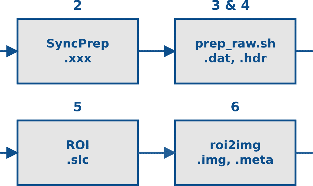
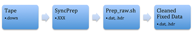
Seasat Processing Project Data Flow: (illustration) Starting with raw signal data on tapes, the Seasat data was successively (1) captured to disk, (2) validated and byte-aligned, (3) decoded, (4) cleaned of bit errors and discontinuities, (5) focused into SLC imagery, (6) processed into georeferenced ground range products, and (7) packaged as HDF5 with XML metadata. Step 2 was performed using the Vexcel product SyncPrep. Step 5 was accomplished using the repeat pass interferometry (ROI) package from JPL. All other steps utilized software developed in-house at ASF.
Written by Tom Logan, July 2013
Seasat – Technical Challenges – 1. Raw Telemetry
Seasat was not equipped with an onboard recorder, so in order to collect data during the mission, three U.S. and two international ground stations downlinked data from the satellite in real time: Fairbanks, Alaska; Goldstone, California; Merritt Island, Florida; Shoe Cove, Newfoundland; and Oakhanger, United Kingdom.
The data were originally archived on 39-track raw data tapes. Years later, to ensure the preservation of the data, those tapes were duplicated in 1988 and again in 1999. During the second transcription, the raw telemetry data were transferred onto 29, more modern SONY SD1-1300L 19-mm tapes. It is from these 13-year-old tapes that ASF’s online Seasat archive was obtained.
An off-the-shelf SAR processor was not available to decode or process Seasat raw telemetry data. However, ASF was able to use the Vexcel product SyncPrep to byte-align the data captured from disk, validate that the data appeared to be Seasat SAR data and estimate the bit error rate (BER) of the data. The BER provided insight into how much of the original SAR data could be processed to products and how difficult that process would be.
In the initial analysis of a 14 GB raw telemetry file, SyncPrep reported bit error rates as high as 0.4, or as many as 1 bit in 2.5 bits in error. This extreme level of “bit rot” persists for much of the Seasat archives and initially seemed to make much of the data unusable. Only through concerted efforts over the course of a year were approximately 90 percent of the Seasat SAR data able to be recovered.
1.1 Minor Frames and Range Lines
The commercial product SyncPrep, used for much of the raw data ingest at ASF, does not decode Seasat telemetry. So while SyncPrep will analyze the data, it will not actually decode metadata or create the range lines needed for focusing the raw data into SAR imagery. Accordingly, a decoder for Seasat raw signal data had to be developed at ASF. First, though, an understanding of the telemetry data format was required.
According to the Interface Control Document for Seasat, the telemetry stream is organized into repeated 1,180-bit telemetry packets, referred to as minor frames. Each minor frame begins with 40 bits of metadata followed by 1,140 bits of payload. The exact subdivision of the minor frames is diagramed below:
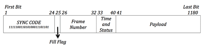
Seasat Raw Telemetry Format: (illustration) Seasat minor frames are comprised of a 24-bit sync code, a 1-bit fill flag, a 7-bit frame number, 8 bits for time and status, and 1,140 bits of payload. The sync code signifies the beginning of each minor frame. The fill flag is supposed to be 1 when no valid data is being sent, 0 if the payload is valid. The frame number allows for sequencing of minor frames and the creation of range lines from them. The time and status bits encode several metadata fields. Finally, the payload contains the actual data samples recorded by the satellite.
The payload in each minor frame is only 1,140 bits. A complete range line of Seasat data consists of the payload from 60 minor frames, each of which contains 228 samples of 5 bits each. So, in order to form range lines from the telemetry data, the payloads from up to 60 minor frames needed to be combined.
Each minor frame number 0 denotes the start of a range line. Minor frame numbers then increase until the start of the next range line, when they are reset to 0.
Aside: Determining Data Size
The pulse repetition frequency (PRF) Rate Code and the Bits Per Sample are required in order to determine the number of minor frames per range line. Seasat had four PRF rate codes: 1: 1464 Hz, 2: 1540 Hz, 3: 1581 Hz, and 4: 1647 Hz. For the entire mission, Seasat stayed with a PRF rate code of 4 and a Bits Per Sample of 5. This should result in 60 to 69 minor frames per range line according to the platform specifications. ASF engineers found that no range line had more than 60 minor frames; they always had either 59 or 60 minor frames. Thus, the output range lines were sized using:
60 minor frames * 1,140 bits/frame * 1 sample/5 bits = 13,680 samples
Thus, 13,680 should be the final size of a single range line once it is decoded into byte samples. For each such range line created, a set of 18 metadata values are also generated.
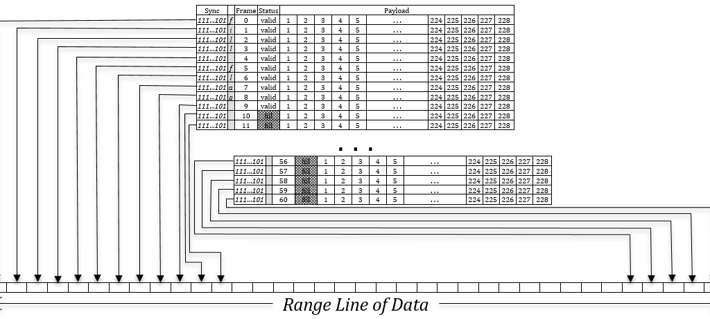
Range Line Creation: (illustration) Creation of a single range line of data requires combining the payload from up to 60 minor frames in order. The 228 samples from minor frame 0 go into the output range line first, followed by the 228 samples from minor frame 1, those from minor frame 2, etc., until all minor frames for this range line have been unpacked. When only 59 frames are in a range line, the remaining 13,680 samples of output for that range line are set to zero. Concurrent with data sample unpacking, image metadata from the Time and Status bits in the first 10 minor frames are decoded and stored.
1.2 Subcommutated Header Fields
The time and status bits encode 18 metadata fields subcommutated in the first 10 minor frames of each range line, i.e. each of these fields need to be created using certain bits from certain numbered minor frames. For example, the Last Digit of Year can be found in bits 33-36 of minor frame 0, giving a range of values from 0-15. Of course, this field should always be 8, as 1978 was the year Seasat was in operation.
The metadata field Day of Year must be created using bits 33-37 of minor frame 4 as the lower-order 5 bits, and bits 37-40 of minor frame 5 as the higher order 4 bits, giving a 9-bit value. Similarly, the MSEC of Day field is 27 bits long and constructed from all or parts of the time and status bytes from minor frames 1-4. The following table shows how each of the 18 metadata fields were created.
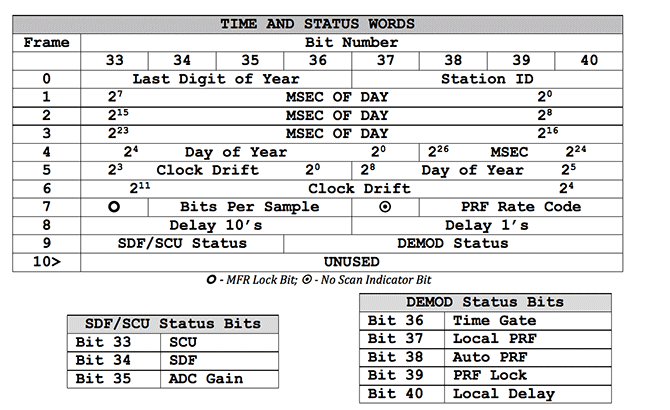
Time and Status Byte: (illustration) Locations of subcommutated metadata values. Only minor frames 0 through 9 contain valid time and status words; in all other minor frames, the time and status word is unused.
| Field | Definition | Type | Notes |
|---|---|---|---|
| Station Code | Signifies which ground station collected the data during the mission | Constant | 5: Fairbanks, AK; 6: Goldstone, CA; 7: Merrit Island, FL; 9: Oak Hangar, United Kingdom; 10: Shoe Cove, Newfoundland. |
| Last Digit of Year | Last digit of the year | Constant | Should always be 8, since the mission was in 1978 |
| Day of Year | Julian day of the year | Rarely | Since no datatakes could possibly be more than a day, this value will change at most once in a datatake. |
| MSEC of Day | Millisecond of the day | Linear | Should change consistently throughout a datatake |
| Clock Drift | Timing offset in spacecraft clock | Curve | Must be added to the other times in order to get proper spacecraft locations |
| No Scan Indicator | Unused | Bit Field | Unused |
| Bits Per Sample | Number of bits per data sample | Constant | Throughout the mission, this value was always 5 |
| MFR Lock Bit | Unused | Bit Field | Unused |
| PFR Rate Code | Pulse Repetition Frequency Code | Constant | Throughout the mission this value was always 4, denoting a PRF of 1647 Hz |
| Delay to Digitization | Delay between sending pulses and when pulses are listened for | Rarely | Used to calculate the slant range to the first pixel in a datatake |
| SCU Bit | Unused | Bit Field | Unused |
| SDF Bit | Unused | Bit Field | Unused |
| ADC Bit | Unused | Bit Field | Unused |
| Time Gate Bit | Unused | Bit Field | Unused |
| Local PRF Bit | Unused | Bit Field | Unused |
| Auto PRF Bit | Unused | Bit Field | Unused |
| PRF Lock Bit | Unused | Bit Field | Unused |
| Local Delay Bit | Unused | Bit Field | Unused |
Metadata Fields in the Raw Data: (table) Eighteen fields of metadata can be decoded for each range line created during decoding. There are 10 bit fields, four fields that should be constant for a datatake, two fields that should change rarely, and two fields that should change steadily.
Written by Tom Logan, July 2013
Seasat – Technical Challenges – 2. Decoder Development
Starting in the summer of 2012, ASF undertook the significant challenge of developing a Seasat telemetry decoder in order to create raw data files suitable for focusing by a synthetic aperture radar (SAR) correlator. In this case, that means processible by ROI, the Repeat Orbit Interferometry package developed at Jet Propulsion Laboratory. In addition to creating the range lines out of minor frames, the decoder must interpret the 18 fields in the headers to create a metadata file describing the state of the satellite when the data was collected.
The main challenges in decoding the raw telemetry were:
- Overcoming bit error problems
- Properly forming major lines from a variable number of minor frames
- Maintaining sync lock
- Discovering sentinels marking data collection boundaries
2.1 Problems with Bit Fields
All 10 of the bit fields proved to be unreliable, and, thus, with the exception of the fill flag, they are ignored by all of the software developed during this project. This section describes the ways in which the bit fields are unreliable.
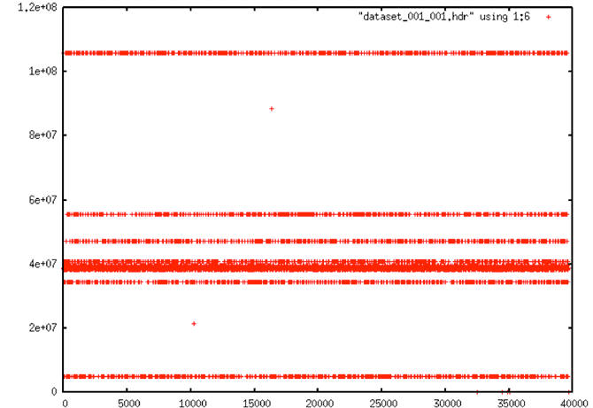
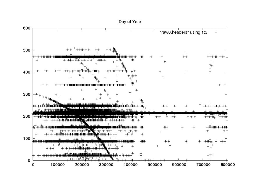
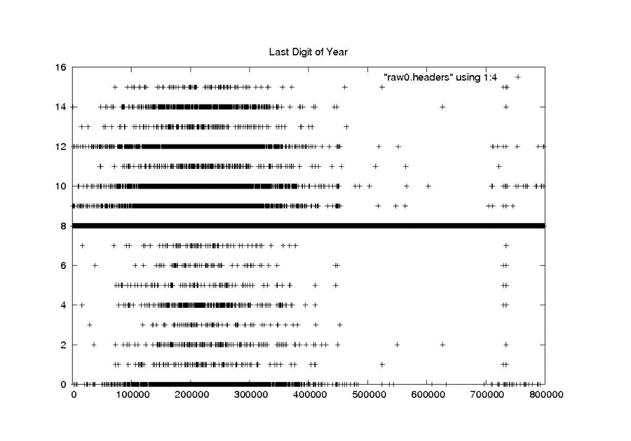
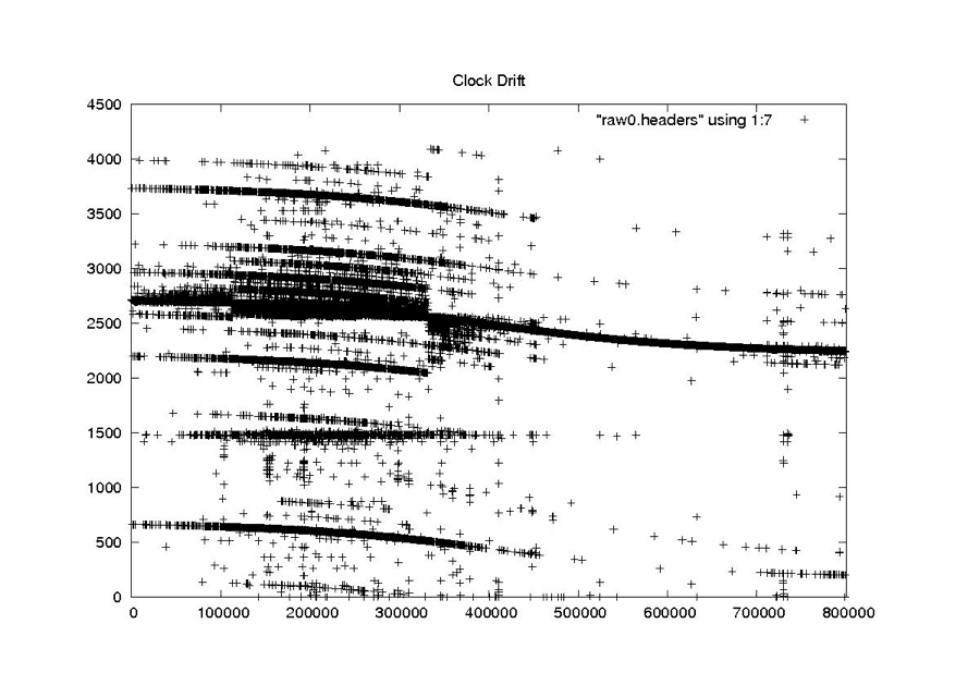
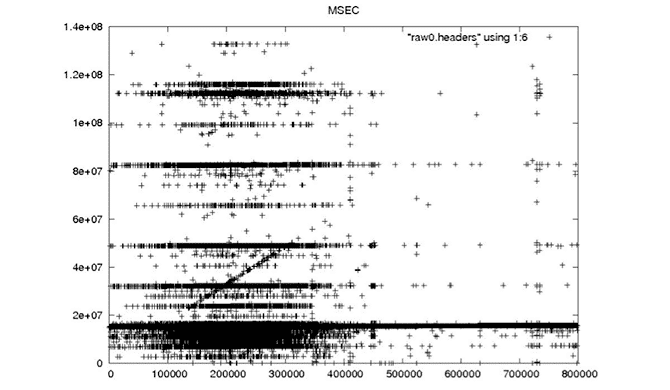
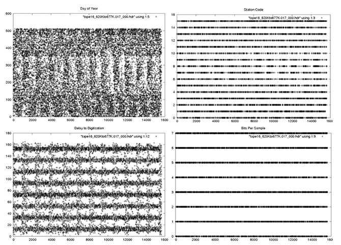
Each Seasat minor frame contains 8 bits to record time and status. These bits encode 18 metadata fields, subcommutated in the first 10 minor frames of each range line. There are 10 bit fields, four fields that should be constant for a data take, two fields that should change rarely and two fields that should change steadily. Unfortunately, due to the high bit error rate (BER) of the telemetry data, even fields that should be constant show high variability. The following plots, showing decoded metadata values plotted over 800,000 range lines, drive home the enormity of the bit error problems in these data.
| Problems with Bit Fields |
|---|
| Bits per Sample |
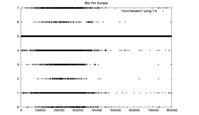 |
| This value should always be 5, as the parameter never changed during the entire Seasat mission. |
| PRF rate code |
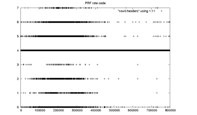 |
| The PRF rate code should be a 4 for the entire mission, since this satellite parameter never changed. |
| Last Digit of Year |
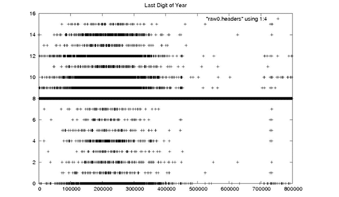 |
| The Seasat mission occurred entirely in 1978, so the last digit of the year should always be 8. |
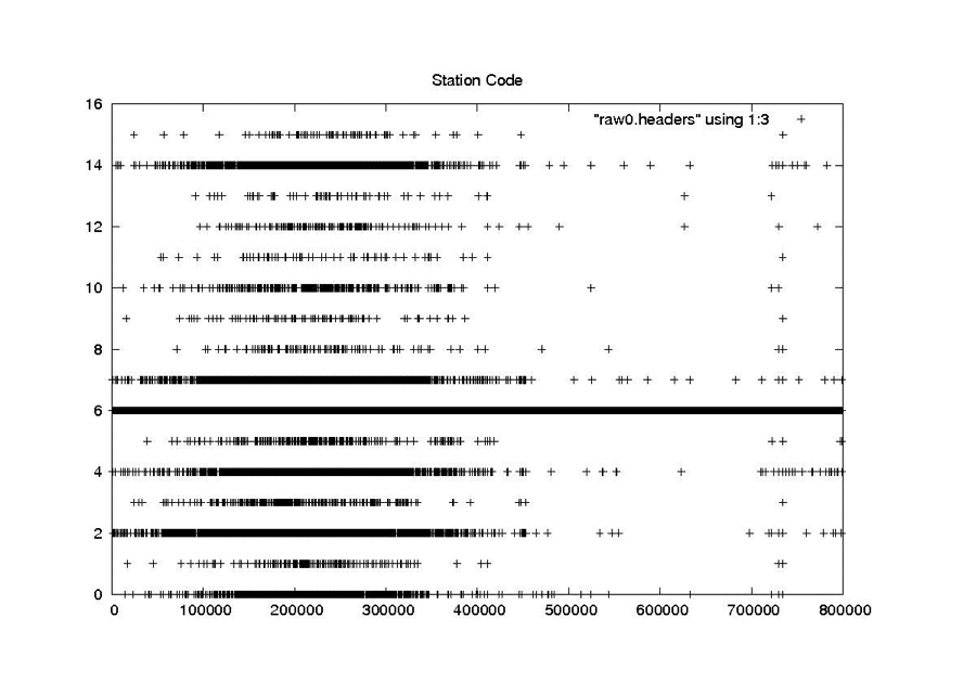
| Station Code |
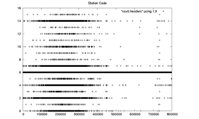 |
| The Station Code should be a constant for any given datatake. 5: Fairbanks, Alaska; 6: Goldstone, Calif.; 7: Merrit Island, Fla.; 9: Oak Hanger, United Kingdom; 10: Shoe Cove, Newfoundland. |
| Day of Year |
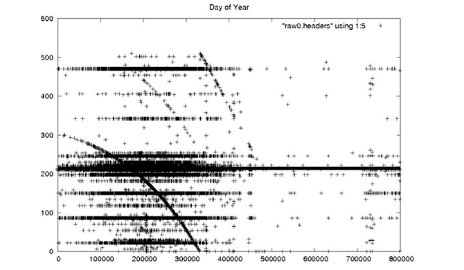 |
| For a given datatake, the day of year should change at most once, since any single datatake cannot exceed even an hour in duration, much less an entire day. |
| Delay to Digitization |
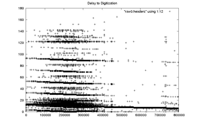 |
| The delay to digitization parameterizes the time between emission of a pulse from the satellite and recording of return echoes. Used to calculate the slant range to the first pixel, the delay should change only a handful of times in any given raw data file based upon changes in orbital altitude. |
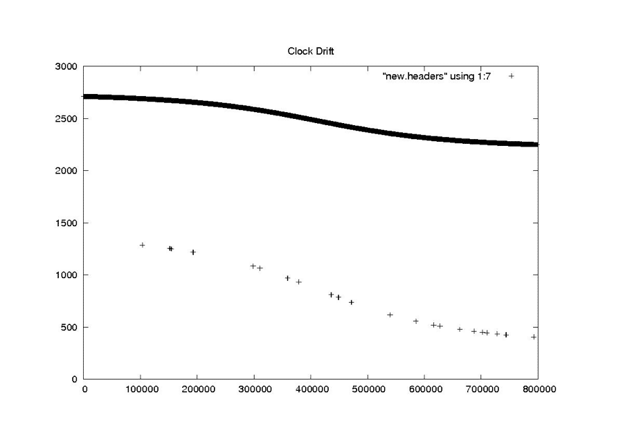
| Clock Drift |
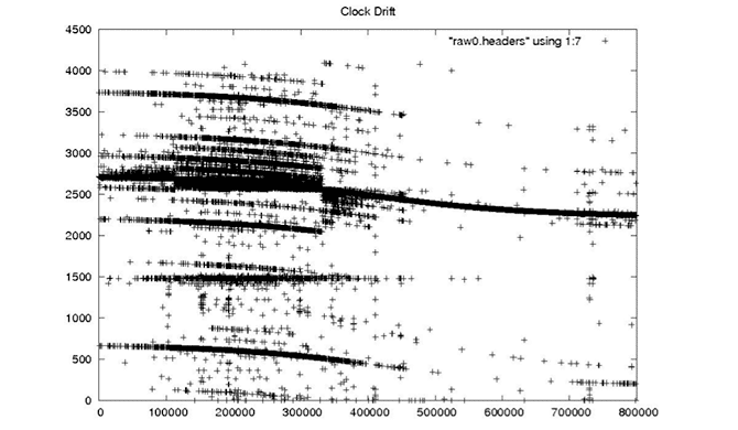 |
| The spacecraft clock drift records the timing error of the spacecraft clock. This should be a smoothly changing field, generally in the 2,000- to 3,000-millisecond range. It is not known how this field was originally created, only that it is vital in getting reasonable geolocations for processed imagery. |
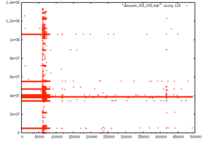
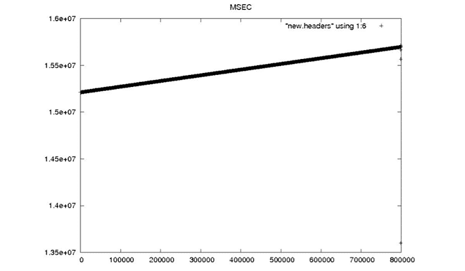
| MSEC |
 |
| This field records the millisecond of the day when the data were acquired and should, therefore, be a linearly increasing field with an exact slope of 1/PRF. |
| Given all of the fallout from these truly bizarre plots, it is no surprise that attempts to use the fill flag quickly proved difficult; the bit errors are so pervasive that the field is unreliable. |
2.2 Determining Minor Frame Numbers
Several oddities in the raw data are exacerbated by the high BER. First, the data are organized into 1,180-bit minor frames. This means that they are each 147.5 bytes long. Although the .5 byte offset was easy to deal with, it turns out that sync codes may actually appear at 147, 147.5, or 148 bytes from each other at seemingly random places in the raw data file – a topic addressed in section 2.3
Moreover, a variable number of minor frames need to be combined to create a single range line. Some lines contain 59 minor frames and some contain 60. Considering that the frame number in the minor frames is only 7 bits, and no major frame numbers exist in the telemetry, the “simple” task of finding the start of each major line was at times quite difficult. Synchronization codes can be either byte-aligned or non-byte-aligned, and partial lines occur on a regular basis. As a result, the minor frame numbers eventually had to be determined by context.
The current frame number is determined using three previous minor frame numbers and the next frame number — along with a handful of heuristics. For example, if a gap is found in consecutive minor frame numbers, the following rules are applied:
- If the next frame is 1 and last was either 59 or 60, assume this is frame zero
- Else if (next_frame-last_frame)==2, put this frame in sequence
- Else if last two frames are in sequence, try to put this one in sequence – If the last frame < 59, put this in sequence – If the last frame was 59 and the last line was length 60, then this HAS to be frame zero since we never have two length 60 lines in a row.
- Else if last2 and last3 frames are in sequence and last frame is 0, then set this frame to 1
- If we got to here, then we did not fix the error!
Even beyond these rules, additional checks for a bad frame number 0 and major frames that spuriously showed more than 60 minor frames still had to be performed.
Aside: Bit Errors in Frame Numbers
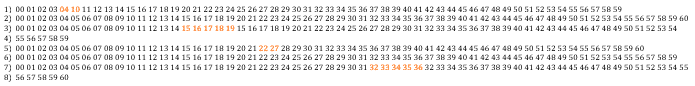
Random bit errors in the middle of a line: In these decoded minor frame numbers, we see that lines 1, 2, 4 and 5 have no frame number errors; they are in sequence starting from 1 and going up to 59 or 60 by ones. Meanwhile, line 3 has 24 frame numbers in a row that are in error.

Partial lines: The first line is missing minor frames 5-9; the second line is complete; the third line has repeated minor frames 15-19; and the fourth line is the decoder’s attempt to enforce the fact that at most 60 minor frames form a range line. The fifth line is missing minor frames 23-26; the sixth line is complete; the seventh line has repeated minor frames 32-36; and, again, the eighth line is the decoder’s attempt to enforce the fact that at most 60 minor frames form a range line.
Multiple lines of bit errors: This example shows how bad random bit errors can be, even if no minor frames are actually missing. Incredibly, in five lines, 122 minor frames are in error out of 298 total, giving a 40 percent error rate for these frame numbers. Perhaps even more incredibly, the ASF Seasat decoder managed to fix all of these frame numbers.
- Original non-fixed frame numbers:

- Frame numbers fixed by the ASF Seasat decoder:

2.3 Maintaining Sync Lock
One very important aspect of decoding telemetry data is maintaining a sync lock: The decoding program must be able to find the synchronization codes that occur at the beginning of each minor frame.
Early in the development of the decoder, it was determined that the sync codes are just as susceptible to bit errors as the rest of the data. Initially, finding sync codes required a considerable amount of searching in the file, with the hope that no false positives would be encountered. After much development and testing, it was determined that in order to maintain sync lock, some number of bit errors had to be allowed in the sync code. Therefore, the code was configured to allow 7 bit errors per sync code out of 24 bits. Values less than this needlessly split datatakes (single passes of data over a given ground station). Values greater than this showed too many “false positive” matches for sync codes.
As a result of this extensive analysis, a pattern was determined in the location of sync codes. That is, a byte-aligned, 147.5-byte frame followed by a non-byte-aligned, 147.5-byte frame, repeated 14,217 times, followed by a single instance of a 147-byte frame. In code form:
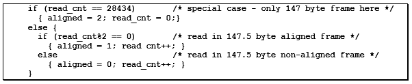
Once this pattern was established, most problems with locating sync codes were abated.
2.4 Data Sentinel Values – Breaking Datatakes
The next problem involved bad sections of data that defied attempts to match frame numbers. The only solution is to break the datatake into multiple pieces, closing the current output file when problems arise, and creating a new output file when sync is regained. This is much like what SyncPrep does, except that the ASF decoder has to be more stringent in its rules for maintaining sync since it must be able to properly build range lines in addition to just finding sync codes.
In addition to losing sync lock as a result of BER, two additional cases arose that will break a datatake into segments: either 60 occurrences of the fill flag in a row, or the repeated occurrence of frame number 127. The fill flag is a valid field but is so unreliable it can only be trusted to be correct after many consecutive hits. The frame number 127 showed to be a sentinel for no data; it occurred thousands of times in areas where no valid SAR data was being collected. Either of these happenings will also cause the ASF Seasat decoder to close the current output file and create a new one.
2.5 Results of Decoding
seasat_decoder:
- Decode raw signal data into unpackaged byte signal data (.dat file)
- 13680 unsigned bytes of signal data per line
- File size is aways lines * 13680 bytes in length
- Decodes all headers to ASCII (.hdr file)
- 20 columns of integer numbers per line
- One line entry per line of decoded signal data
- Additional Features:
- Allows both byte aligned and anon-byte aligned minor frames
- Deals with variable length lines, partial lines
- Fixes frame numbers from context if possible
- Creates one or more output files per input based on sentinels
- Assembles headers spread across 10 minor frames
In spite of all of the challenges and problems in the raw data, the ASF Seasat decoder is able to decode raw telemetry SAR data. Using five frame numbers in sequence and a handful of heuristics, telemetry data is decoded into byte-aligned, 8-bit samples. Concurrently, all of the metadata stored in the headers is decoded and placed in an external file.
The current strategy tried to err on the side of only allowing valid SAR data to be decoded. Still, 7-bit errors had to be allowed in a sync code match to even get through the raw data. In addition, the decoded header information is simply not reliable. For example, early in development, the ASF Seasat decoder broke one 7-GB chunk of raw data into 24 segments of decoded data, dumping a header at the beginning and ending of each segment. Analysis of the decoded times in these headers showed that of the 48 dumped, 3 were completely zero and an additional 12 were in error. In other words, the decoded times did not make sense in context with the surrounding time values.
Thus, even after completing the decoder development with bit error tolerance, frame number heuristics, proper sync code detection, and known sentinel values for good data boundaries, the decoded Seasat archives were still nearly unusable in any reliable fashion.
| Processing Stage | #Files | Size (GB) |
|---|---|---|
| Capture | 38 | 2610 |
| SyncPrep | 1840 | 2431 |
| Original Decoded | 1470 | 3585 |
Initial Data Recovery: (table) 93 percent of the data captured from tape made it through SyncPrep; Approximately 92 percent of that data was decoded (assuming a 1.6-expansion factor).
Aside: ASF Tape Archive File Names
When the tapes were captured onto disk, files were named based upon tape number and section of tape read. For example, the first part of tape1 was initially named SEASAT_tape1_01Kto287K.
This file was run through SyncPrep, which created multiple subfiles based upon its ability to maintain a sync lock, sometimes creating over 100 such numbered files, e.g. SEASAT_tape1_01Kto287K.000 to SEASAT_tape1_280Kto668K.020
Next, the files go through the ASF Seasat decoder, gaining yet another subfile number, but the prefix “SEASAT_” is removed. Note that this stage creates a file pair of {.dat, .hdr}, e.g. tape1_01Kto287K.018_000, tape1_01Kto287K.018_001, and tape1_01Kto287K.018_002 file pairs were all created from a single decode of SEASAT_tape1_280Kto668K.018.
Thus, for a single captured file, SyncPrep could make tens to a few hundred data segments, while the ASF Seasat decoder could break each of these files into even more sub-segments.
Written by Tom Logan, July 2013
With the Seasat archives decoded into range line format along with an auxiliary header file full of metadata, the next step is to focus the data into synthetic aperture radar (SAR) imagery. Focusing is the transformation of raw signal data into a spatial image. Unfortunately, pervasive bit errors, data drop outs, partial lines, discontinuities and many other irregularities were still present in the decoded data.
3.1 Important Metadata Fields
In order for the decoded SAR data to be focused properly, the satellite position at the time of data collection must be known. The position and velocity of the satellite are derived from the timestamp in each decoded data segment, making it imperative that the timestamps are correct in each of the decoded data frames.
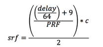
Slant range is the line of sight distance from the satellite to the ground. This distance must be known for focusing reasons and for geolocation purposes. As the satellite distance from the ground changes during an orbit, the change is quantified using the delay-to-digitization field. During focusing, the slant range to the first pixel is calculated using these quantified values. More specifically, the slant range to the first pixel (srf) is determined using the delay to digitization (delay), the pulse repetition frequency (PRF) and the speed of light (c):
It turns out that the clock drift is also an important metadata field. Clock drift records the timing error of the spacecraft clock. Although it is not known how this field was originally created, upon adding this offset to the day of year and millisecond of day more accurate geolocations were obtained in the focused Seasat products.
Finally, although not vital to the processing of images, the station code provides information about the where the data was collected and may be useful for future analysis of the removal of systematic errors.
3.2 Bit Errors
It is assumed that the vast majority of the problems in the original data are due to bit errors resulting from the long dormancy of the raw data on magnetic tapes. The plots in section 2.1 showed typical examples of the extreme problems introduced by these errors, as do the following time plots.
| Bit Errors |
|---|
| It is assumed that the vast majority of the problems in the original data are due to bit errors resulting from the long dormancy of the raw data on magnetic tapes. The plots in section 2.1 showed typical examples of the extreme problems introduced by these errors, as do the following time plots. |
 |
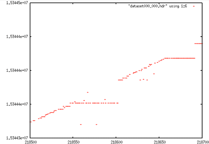
| Time Plot: Very regular errors occur in much of the data, almost certainly some of which are due strictly to bit errors. Note that this plot should show a slope, but the many errors make it look flat instead. |
 |
| Time Plot: This plot shows a typical occurrence in the Seasat raw data: Some areas of the data are completely fraught with random errors; other areas are fairly “calm” in comparison. |
3.3 Systematic Errors in Timing
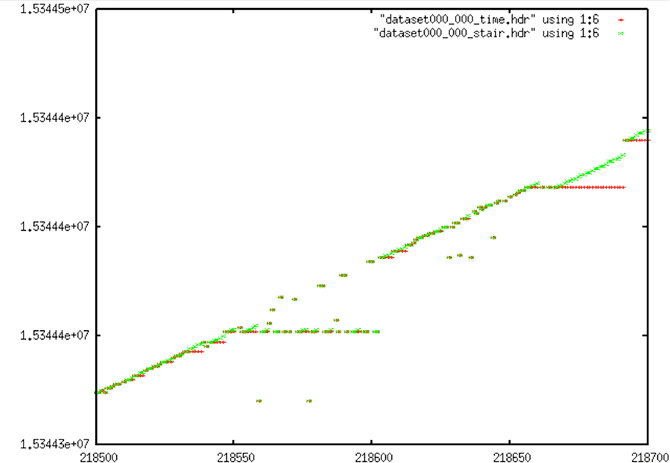
Beyond the bit errors, other, more systematic errors affect the Seasat timing fields. These include box patterns, stair steps and data dropouts.
To top off the problems with the time fields, discontinuities occur on a regular basis in these files. Some files have none; some have hundreds. Some discontinuities are small — only a few lines. Other discontinuities are very large — hundreds to thousands of lines. Focusing these data required identifying and dealing with discontinuities.
| Systematic Errors in Timing |
|---|
| Box errors |
 |
| Stair Steps |
 |
| Data Dropouts |
 |
| Forward Time Discontinuity |
 |
| Backward Time Discontinuity |
 |
| Double Discontinuity |
 |
| Time Discontinuity |
 |
Aside: Initial Data Quality Assessment
Of the 1,470 original decoded data swaths
- Datasets with Time Gaps (>5 msec): 728
- Largest Time Gap: 54260282
- Largest Number of Gaps in a Single File:1,820
- Number of files with stair steps: 295
- Largest percentage of valid repeated times: 63%
- Number of files with more than one partial line: 1,170
- Largest percentage of partial lines: 42%
- Number of files with bad frame numbers: 1,470
- Largest percentage of bad frame numbers: 17%
Seasat – Technical Challenges – 4. Data Cleaning (Part 1)
In order to create a synthetic aperture for a radar system, one must combine many returns over time. For Seasat, a typical azimuth reference function — the number of returns combined into a single focused range line — is 5,600 samples. Each of these samples is actually a range line of radar echoes from the ground. Properly combining all of these lines requires knowing precisely when a range line was received by the satellite.
In practice, SAR systems transmit pulses of energy equally spaced in time. This time is set by the pulse repetition frequency (PRF); for Seasat, 1,647 pulses are transmitted every second. Alternatively, it can be said a pulse is transmitted every 0.607165 milliseconds, an interval commonly referred to as the pulse repetition interval or PRI. Without this constant time between pulses, the SAR algorithm would break down and data would not be focused to imagery.
Many errors existed in the Seasat raw data decoded at ASF. As a result, multiple levels of filtering were required to deal with issues present in the raw telemetry data, particularly with time values. Only after this filtering were the raw SAR data processible to images.
4.1 Median Filtering and Linear Regression
The first attempt at cleaning the data involved a simple one-pass filter of the pertinent metadata parameters. The following seven parameters were median filtered to pull out the most commonly occurring value: station code, day of year, clock drift, delay to digitization, least significant digit of year, bits per sample and PRF rate code. A linear regression was used to clean the MSEC of Day metadata field. This logic is encapsulated in the program fix_headers, which is discussed in more detail in “Final Form of Fix_Headers.”
Implementing the median filter was straightforward:
- Read through the header file and maintain histograms of the relevant parameters.
- Use the local median value to replace the decoded value and create a cleaned header file. Here “local” refers to the 400 values preceding the value to be replaced.
This scheme works well for cleaning the constant and rarely changing fields. It also seems to work quite well for the smoothly changing clock drift field. At the end of this section are the examples from “Problems with Bit Fields,” along with the corresponding median-filtered versions of the same metadata parameters. In each case, the median filter created clean usable metadata files.
Performing the linear regression on the MSEC of Day field was also straightforward. Unfortunately, the results were far from expected or optimal. The sheer volume of bit errors combined with discontinuities and timing dropouts made the line slopes and offsets highly variable inside a single swath. These issues will be examined in the next section.
Table of Filtered Parameters
| Parameter | Filter Applied | Value |
|---|---|---|
| station_code | Median | Constant per datatake |
| day_of_year | Median | Varies |
| clock_drift | Median | Varies |
| delay_to_digitization | Median | Varies |
| least_significant_digit_of_year | Median | 8 |
| bit_per_sample | Median | 5 |
| prf_rate_code | Median | 4 |
| msec_of_day | Linear Regression | Varies |
Data Cleaning Examples
| Data Cleaning Examples |
|---|
| Station Code |
 |
| Seasat – Station Code – Raw Headers |
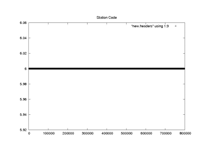 |
| Seasat – Station Code – New Headers |
| Day of Year |
 |
| Seasat – Day of Year – Raw Headers |
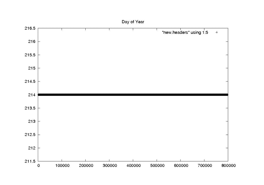 |
| Seasat – Day of Year – New Headers |
| Last Digit of the Year |
 |
| Seasat – Last Digit of the Year – Raw Headers |
 |
| Seasat – Last Digit of the Year – New Headers |
| Clock Drift |
 |
| Seasat – Clock Drift – Raw Headers |
 |
| Seasat – Clock Drift – New Headers |
| Bits Per Sample |
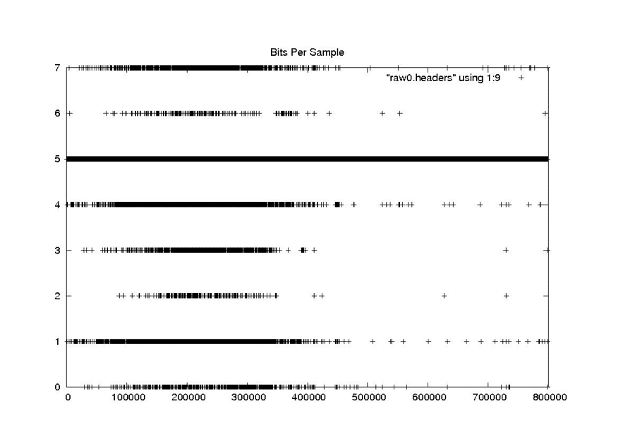 |
| Seasat – Bits Per Sample – Raw Headers |
 |
| Seasat – Bits Per Sample – New Headers |
| PRF Rate Code |
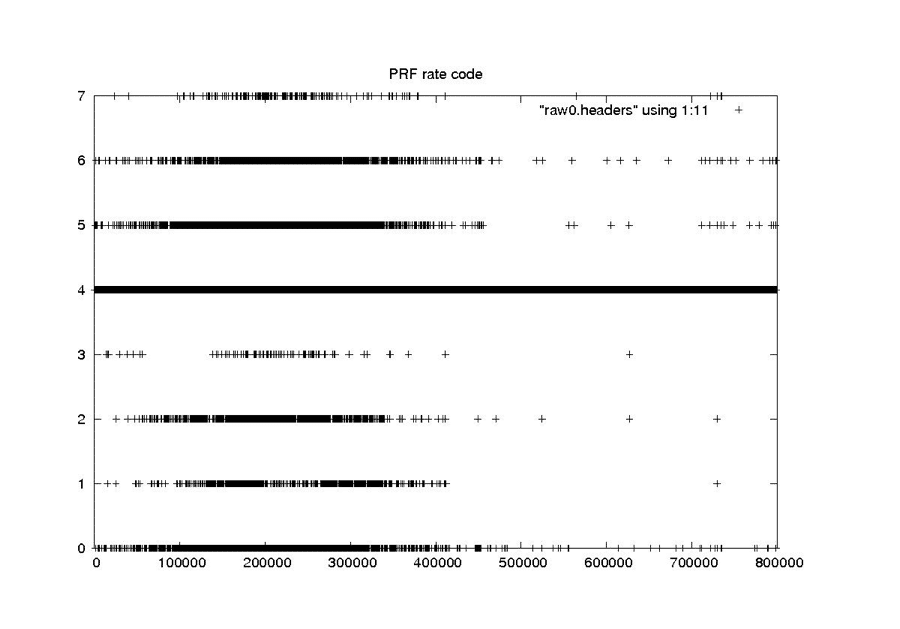 |
| Seasat – PRF Rate Code – Raw Headers |
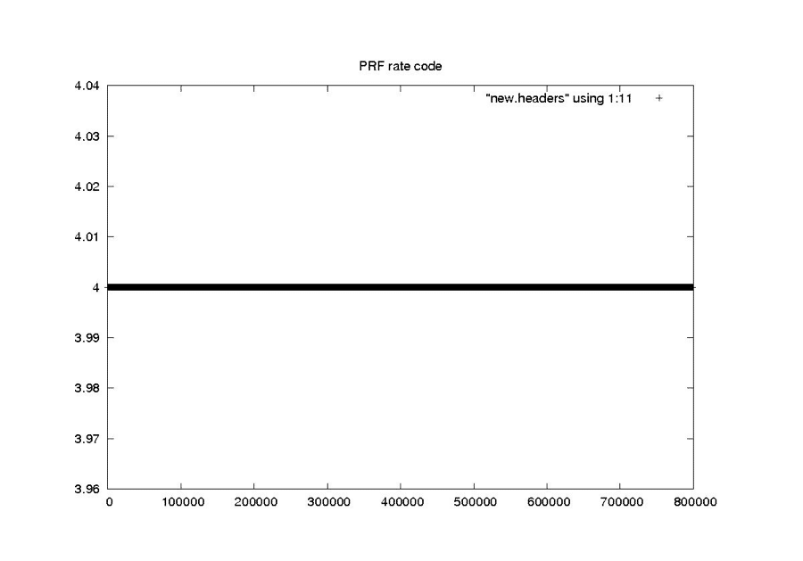 |
| Seasat – PRF Rate Code – New Headers |
| Delay to Digitzation |
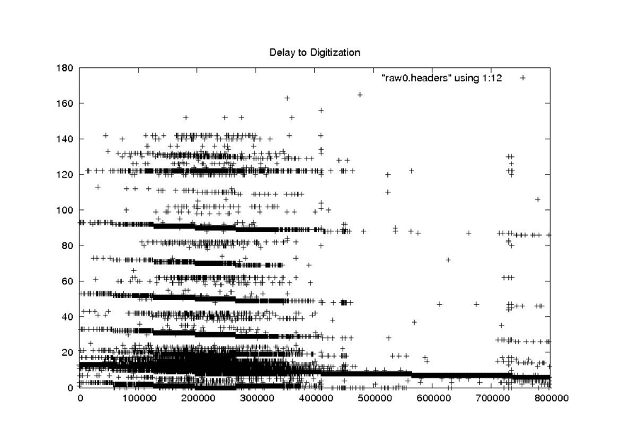 |
| Delay to Digitization – Raw Headers |
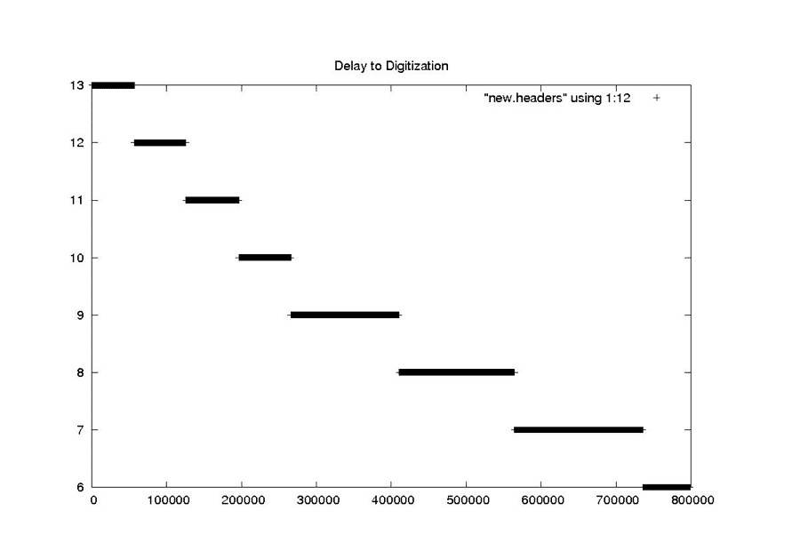 |
| Seasat – Delay to Digitization – New Headers |
4.2 Time Cleaning
Creating a SAR image requires combining many radar returns over time. This requires that very accurate times are known for every SAR sample recorded. In the decoded Seasat data, the sheer volume of bit errors, combined with discontinuities and timing dropouts, resulted in highly variable times inside a single swath.
4.2.1 Restricting the Time Slope
One of the big problems with applying a simple linear regression to the Seasat timing information was that the local slope often changed drastically from one section of a file to another based upon bit errors, stair steps and discontinuities. Since a pulse is transmitted every 0.607165 milliseconds, it seemed that the easiest way to clean all of the MSEC times would be to simply find the fixed offset for a given swath file and then apply the known time slope to generate new time values for a cleaned header file.
This restricted slope regression was implemented when it became obvious that a simple linear regression was failing. By restricting the time slope of a file to be near the 0.607-msec/line known value, it was assumed that timing issues other than discontinuities could be removed. The discontinuities would still have to be found and fixed separately in order for the SAR focusing algorithm to work properly. Otherwise, the precise time of each line would not be known.
4.2.2 Removing Bit Errors from Times
fix_time
Crude time filtering, trying to fix all values that are > 513 from local linear trend:
Bit fixes – replace values powers of 2 from trend
Fill fixes – fill gaps in constant consecutive values
Linear fixes – replace values with linear trend
Reads and writes a file of headers
Even with linear regressions and time slope limitations, times still were not being brought into reasonable ranges. Too many values were in error in some files, and a suitable linear trend could not be obtained. So, another layer of time cleaning was added as a pre-filter to the final linear regression done in fix_headers. The program fix_time was initially created just to look for bit errors, but was later expanded to incorporate each of three different filters at the gross level (i.e. only values > 513 from a local linear trend are changed):
- If the value is an exact power of 2 off from the local linear trend, then add that power of 2 into the value. This fix attempts to first change values that are wrong simply because of bit errors. The idea is that this is a common known error type and should be assumed as the first cause.
- Else if the value is between two values that are the same, make it the same as its neighbors. This fix takes advantage of the stair steps found in the timing fields. It was only added in conjunction with the fix_stairs program discussed below. The idea is to take advantage of the fact that the stair steps are easily corrected using the known satellite PRI.
- Else just replace the value with the local linear trend. At this point, it is better to bring the points close to the line than to leave them with very large errors.
4.2.3 Removing Stair Steps from Times
fix_stairs
Fix for sticky time field – Turns “stairs” into “lines” by replacing repeated time values with linear approximation for better linear trend
Reads and writes a file of headers
For yet another pre-filter, it was determined that the stair steps time anomaly should be removed before fitting points to a final linear trend. This task is relatively straightforward: If several time values in a row are the same, replace them with values that fit the known time slope of the satellite. The program fix_stairs was developed to deal with this problem.
4.2.4 Final Form of fix_headers
fix_headers
- Miscellaneous header cleaning using median filters:
- Station Code
- Least Significant Digit of Year
- Day of Year
- Clock Drift
- Bits Per Sample
- PRF Rate Code
- Delay to Digitization
- Time Discontinuity Location and Additional Filtering
- Replace all values > 2 from linear trend with linear trend
- Locates discontinuities in time, making an annotated file for later use.
- 5 bad values with same offset from trend identity a discontinuity
- +1 discontinuity is forward in time and can be fixed
- if > 4000, too large – cannot be fixed
- otherwise, slide time to fit discontinuity
- if offset > 5 time values, save this discontinuity in a file
- -1 discontinuity is backwards in time and cannot be fixed
- Reads and writes a file of headers
Although it started out as the main cleaning program, fix_headers is currently the final link in the cleaning process. Metadata going through fix_headers has already been partially fixed by reducing bit errors, removing stair steps, and bringing all other values that show very large offsets into a rough linear fit. So in addition to performing median filtering on important metadata fields (see section 4.1), this program performs the final linear fit on the time data.
Initially, a regression is performed on the first window of 400 points and used to fix the first 200 time values of that window. Any values that are more than 5 msec from their predecessors are replaced by the linear fit. After this, a new fit is calculated every window/2 samples, but never within 100 samples of an actual discontinuity. The final task for fix_headers was to locate the rough locations of all real discontinuities that occur in the files. At least, it was designed to only find real discontinuities – those being the final problem hindering the placement of reasonable linear times in the swath files.
Identifying discontinuities was challenging. Much trial and error resulted in a code that worked for nearly all cases and was able to be configured to work for the other cases as well. The basic idea is that if a gap is found in the data, and if after the gap no other gaps occur within 5 values, then it is possible that a discontinuity exists. If so, the program determines the number of lines that would have to be missing to create such a gap and records the location and size in an external discontinuity file. Note that only forward discontinuities can be fixed in this manner and only discontinuities less than a certain size. In practice, the procedure attempts to locate gaps of up to 4,000 lines, discarding any datasets that show gaps larger than this.
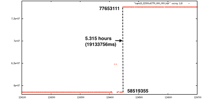
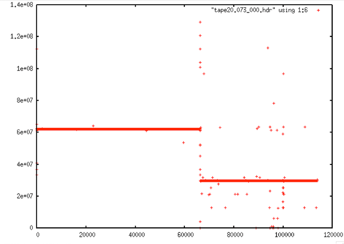
Extreme Discontinuity: This decoded signal data shows a 5.3-hour gap in time. This cannot be fixed.
In the end, all of the gaps in the data were identified, and, there is high confidence that any such discontinuities found are real and not just the result of bit errors or other problems. Unfortunately, this method was not able to pinpoint the start of problems, only that they existed, as shown in the following set of graphs.
| Set of graphs |
|---|
| Decoded Signal Data with No Y-range Clipping |
 |
| Decoded Signal Data with No Y-range Clipping: As usual, if all times from a metadata file are plotted, there are so many errors that the time line looks flat even though it must have a slope around 0.607 by definition. From this plot, it is not obvious that this data even has a discontinuity, much less what the location may be. |
| Decoded Signal Data with Y-range Clipping |
 |
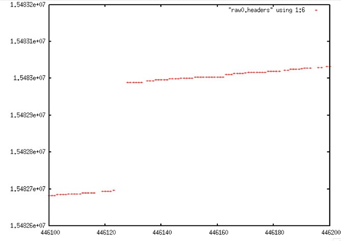
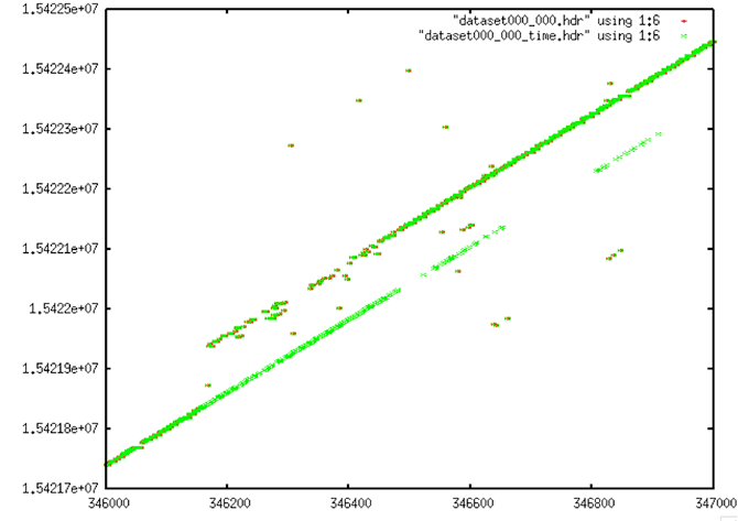
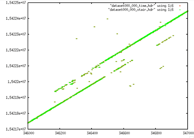
| Decoded Signal Data with Y-range Clipping: When a specific section of the time values are plotted, a clearer picture emerges. The data show dropouts, bit errors and a discontinuity |
| Linear Trend of Decoded Signal Data |
 |
| Linear Trend of Decoded Signal Data: This graph shows the bad time values being replaced by good values using the linear trending technique employed by fix_headers. |
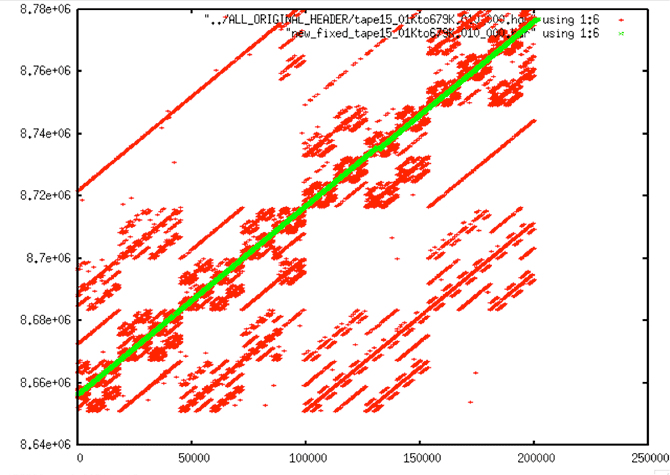
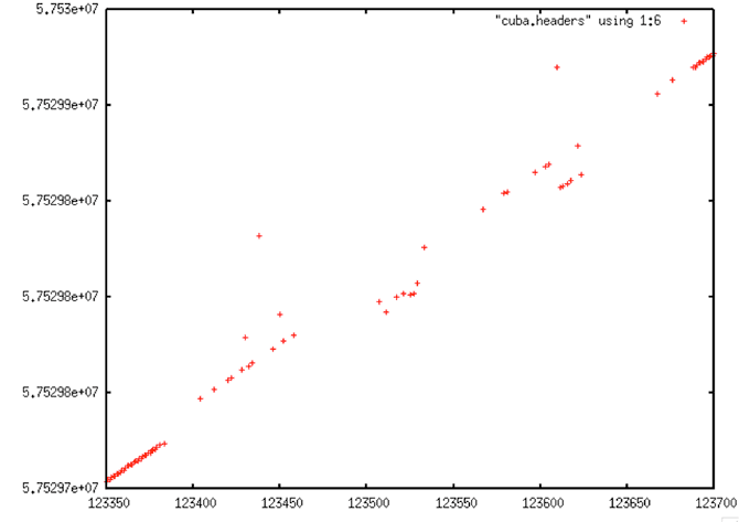
| Comparison of Decoded Signal Data and Linear Fit |
 [ [ |
| Comparison of Decoded Signal Data and Linear Fit: In this plot, it is visually obvious that the linear trend is not switching over for some 350 lines past where it should. But, given how sparse the reasonable data is from 123400 to 123680 or so, it was not clear if it would ever be feasible to get this correct algorithmically. |
| False Discontinuity #1 |
 |
| False Discontinuity #1: Due to high BER, the search program faced many challenges like this, in which a forward discontinuity was “found,” followed closely by a reverse discontinuity. The problem was overcome only after much trial and error with processing parameters. |
| False Discontinuity #2 |
 |
| False Discontinuity #2: Another example of a false discontinuity “discovered” by the ASF cleaning software. Because no reverse time discontinuities can be fixed, this file initially had a false discontinuity inserted. The problem was overcome only after much trial and error with window sizes, gap lengths, gap shifts allowed and other processing parameters. |
4.2.5 Removing Discontinuities
dis_search
- fix all time discontinuities in the raw swath files
- for each entry in previously generated discontinuity file:
- search backwards from discontinuity looking for points that don’t fit new trend line
- when 20 consecutive values that are ont within 1.5 of new line are found, you have found start of discontinuity
- For length of discontinuity
- Repeat header line in .hdr file (fixing the time only)
- Fill .dat file with random values
- Reads discontinuity file, original .dat and .hdr file, and cleaned .hdr file. Creates final cleaned .dat and .hdr file ready for processing
The first task in removing the discontinuities is locating them. The rough area of each real discontinuity can be found using the fix_headers code as described in the previous section.
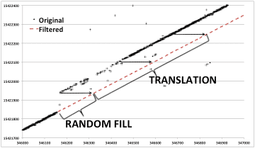
Finding the exact start and length of each discontinuity still remains to be done. This search and the act of filling each gap thus discovered is performed by the program dis_search. The discontinuity search is performed backward, with 3000 lines after each discontinuity area being cached and then searched for a jump down in the time value to the previous line. These locations were marked as the actual start of the discontinuity. The gap in the raw data between the time before the discontinuity and the time after must then be filled in. Random values were used for fill, these being the best way to not impact the usefulness of the real SAR data.
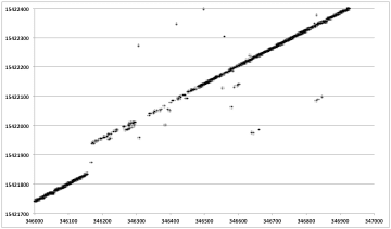
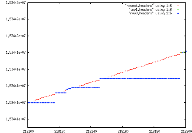
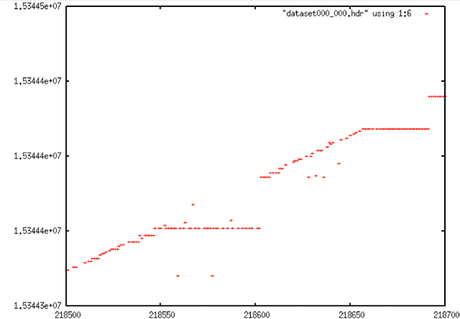
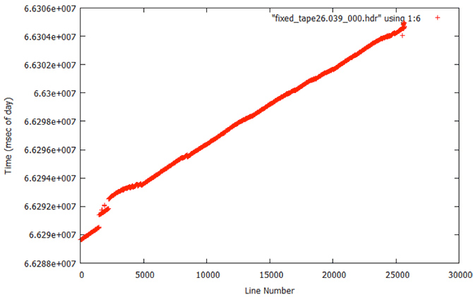
Discontinuity Fills: Each plot shows range line number versus MSEC metadata value. Original decoded metadata is spotty and contains an obvious time discontinuity.
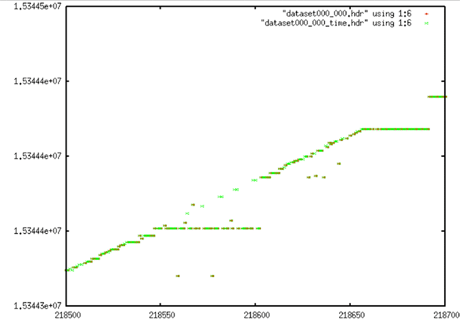
Discontinuity Fills: Each plot shows range line number versus MSEC metadata value. After the discontinuity is found and corrected, linear time is restored.
Seasat – Technical Challenges – 4. Data Cleaning (Part 2)
4.3 Prep_Raw.sh
After development of each of the software pieces described previously in this section, the entire data cleaning process was driven by the program prep_raw.sh. This procedure was run on all of the swaths that were output from SyncPrep to create the first version of the ASF online Seasat raw data archive (the fixed_ files). Analysis of these results is covered in the next section. What follows here are examples of the prep_raw.sh process and intermediate outputs.
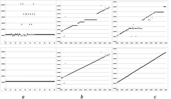
Time Filtering in Stages: Each plot shows range line number versus MSEC metadata value. Top row is before filtering; bottom is after. From left to right: (a) Stage 1 — attempt to fix all time values > 513 from the linear trend. (b) Stage 2 — fix stair steps resulting from sticking clock on satellite. (c) Stage 3 — final linear fix before discontinuity removal.
Data Set #1
| Data Set #1 |
|---|
| Decoded Signal Data |
 |
| Data contain lots of bit errors, dropouts and stair steps. |
| Time Gap Corrections |
 |
| Time Gap Corrections: A few large bit errors and some fill fixes have been applied. |
| Stair Corrections |
 |
| Stair Corrections: A few of the stairs in this image have been partially corrected. |
Data Set #2
| Data Set #2 |
|---|
| Decoded Signal Data |
 |
| This shows a typical discontinuity situation. The data at the crossover from before to after the gap is spotty, filled with bit errors and dropouts. (Image is identical to seasat_decoded_signal_data_1) |
| Time Gap Corrections |
 |
| Time Gap Corrections: Gaps in the data have mostly been filled in. Some are incorrect – particularly the green values that match the lower line but are on the right side of this plot. |
| Stair Corrections |
 |
| Stair Corrections: Since no stair step anomaly exists in this data, there is no visual change here. |
| Linear Time Restored |
 |
| Linear Time Restored: After the discontinuity is filled, linear time is restored in this file. |
| Decoded Time Data from Section 2.1 Examples |
 |
| Cleaned Time Data from 2.1 Examples |
 |
4.4 Results of Prep_Raw.sh
By November 15, 2012, the beta version of prep_raw.sh was delivered to ASF operations. It was run on individual swaths at first, with results spot-checked. Once confidence in the programs increased, all remaining Seasat swaths were processed through this decoding and cleaning software en masse. Overall, from the 1,840 files that SyncPrep created, 1,470 were successfully decoded, and 1,399 of those made it through the prep_raw.sh procedure to create a set of fixed decoded files. The files that failed comprise 242 GB of data, while 3,318 GB of decoded swath data files were created.
| Processing Stage | #files | Size (GB) |
|---|---|---|
| Capture | 38 | 2160 |
| SyncPrep | 1840 | 2431 |
| Original Decoded | 1470 | 3585 |
| Fixed Decoded | 1399 | 3318 |
| Good Decoded | 1346 | 3160 |
| Bad Decoded | 53 | 157 |
Summary of Data Cleaning
93% of data made it through SyncPrep
92% of that data decoded (assume 1.6 expansion)
93% of that data was “fixed”
95% of that data considered “good”
OVERALL: ~80% of SyncPrep’d data is “good”
Reasons for Failures
- SyncPrep: Not all captured files could be interpreted by SyncPrep
- Original Decoded: Because the decoder needs to interpret the subcommutated headers, it is more stringent on maintaining a “sync lock” than SyncPrep
- Fixed Decoded: Some files are so badly mangled that a reasonable time sequence could not be recovered
- Bad Decoded: Several subcategories of remaining data errors are discussed in section 5
4.5 Addition of fix_start_times
During analysis of the fixed metadata files, it was discovered that bad times occurred at the beginning of many files. This problem was not a big surprise; the nature of the sync code search is such that many errors occur in places where the sync codes cannot be found. This is why the files were broken in the first place. So, it is expected that the beginning of a lot of the swath files will have bad metadata, which means bad times. When bad times are linearly trended, the results are unpredictable.
Bad Start Time Examples
| Bad Start Time Examples |
|---|
 |
| Bad Start Time: Many of the bad start times can be readily observed in plots. In this case the trend started at zero time with a huge slope. It is not until after the first window of data that a reasonable line is found to fit the data. |
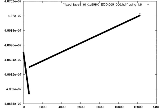 |
| Bad Start Time: In this case, a reverse time slope is shown at the start of the file. |
 |
| Bad Start Time: In this extreme case, a reverse time slope resulted from bad linear trending at the start of this file and continued in error for the entire rest of the file. |
To fix this problem, yet another level of filtering was added to the processing flow – this time a post-filter to fix the start times. The code fix_start_times replaces the first 5,000 times in a file with the linear trend resulting from the next 10,000 lines in the file. This code was added as a post-processing step to follow prep_raw.sh and run on all of the decoded swath files.
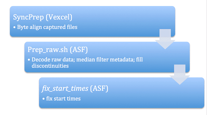
Final Processing Flow: (illustration) With the addition of the fix_start_times code, the processing flow for data decode and cleaning is finally completed.
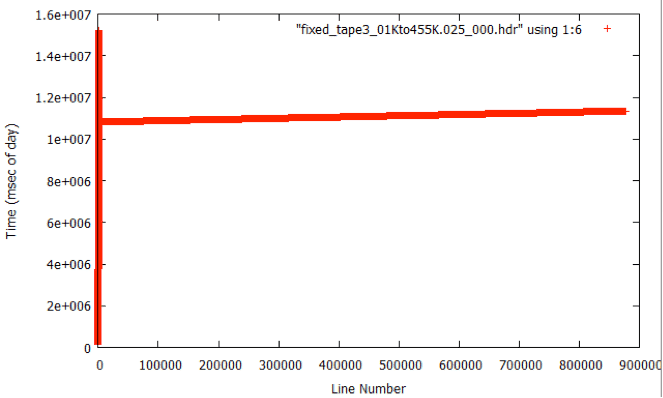
Fixed Start Time Examples
| Fixed Start Time Examples |
|---|
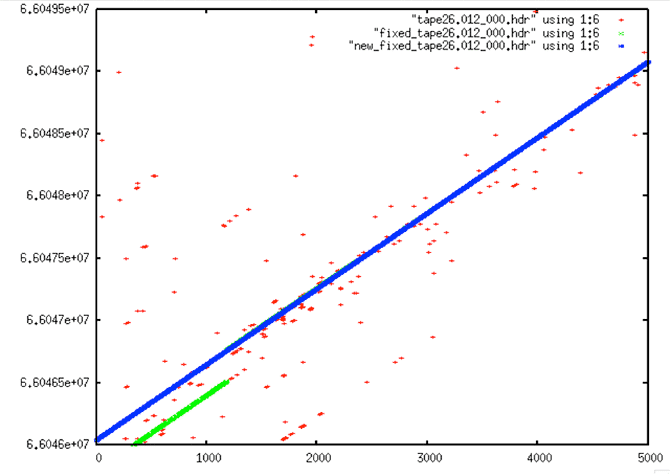 |
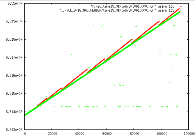
| Fixed Start Time #1: In this example, the original data (red) doesn’t look that bad. However, the first attempt at cleaning (green) gave wrong start values. Only after running fix_start_times were the times forced to a reasonable linear progression. |
 |
| Scatter chart |
 |
| Fixed Start Time #3: The original data here (red) is quite sparse at the start of this swath. The first fix (green) is obviously very wrong. However, as before, when the start times are fixed, the resulting times are a clean line. |
Written by Tom Logan, July 2013
Seasat – Technical Challenges – 5. Classification of Bad Data
In spite of all of the work done to decode and clean data, many errors remained in the supposedly fixed files that had been decoded and multi-pass filtered. As a result, the current count for swath files able to be processed is 1,346 rather than the 1,399 that first came out of prep_raw.sh. Each of these classes of errors are discussed in this section.
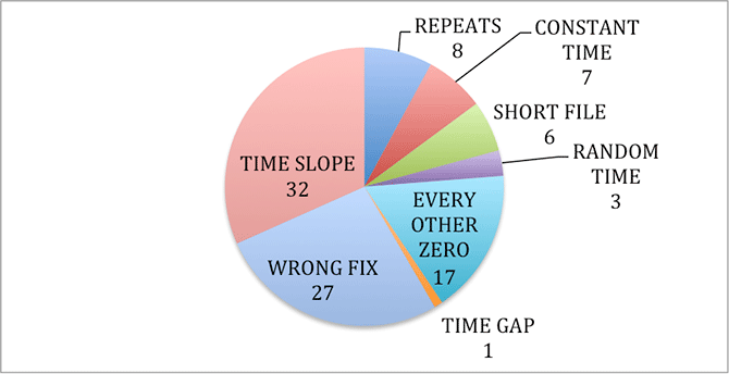
Classification of Bad Data: (illustration) Initially 101 files were discarded. One category, repeats, was simply the result of one tape portion being read twice. Eight duplicate files were discarded.
5.1 Short Files
Six files fewer than 10,000 lines long were discovered and removed from the processing set. The number of lines needed to create a 100-km length frame was later determined to be 24,936. Thus, even more files could be removed since they will not create full frames.
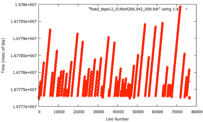
5.2 Constant Time
Seven different files from Tape12 all have a constant time of 16777216 throughout. Obviously, this data could not be processed and was discarded. Also, the first five files of tape10 had values of 134217727, but these were discarded during the initial data prep.
5.3 Random Time
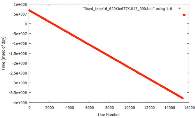
Three files were identified with nearly random time values. Again, due to the nature of SAR processing, these files were not used. Those files were fixed_tape16_620Kto677K.017_000.hdr, fixed_tape26.039_000.hdr, and fixed_tape28.002_000.hdr.
Constant Time: When the fix routines were applied to a file with constant times, this is the result. Because the codes are trying to fit the times to a “known” slope when none actually exists in the data, spurious times are introduced.
Random Times: Metadata plots of one file from the Random Time error category.
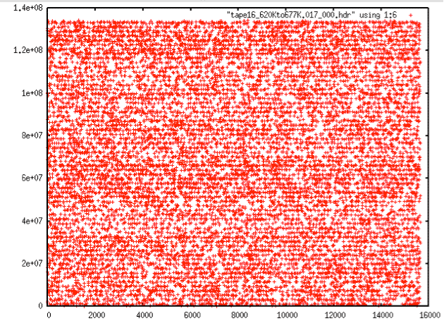
Random Times: Time plot of one file from the Random Time error category showing decoded MSECs vs. range line. This data cannot be recovered.
5.4 Every Other Zero
Seventeen files were found with some number of headers that contained only zero values. With 1 percent all the way up to 100 percent of the metadata in these files being blank, they were removed from the data set.
5.5 Time Gap
One file was found with a very large time gap that was unable to be fixed. It was removed.
5.6 Time Slope
Based upon slope analysis, thirty-two files were marked as having an incorrect time slope. This was the beginning of the realization that something was wrong with the Seasat time fields. This is discussed in full in section 6, “Tackling the Slope Issues.” This class of errors was revisited and the number was reduced to a mere six swaths that didn’t process correctly.
5.7 Wrong Fix
Initially, 27 files were placed in the wrong fix category based upon visual inspection of the supposedly fixed files. It turns out that these resulted from the time slope assumptions that were built into all of the software. In other words, all of the programs that did linear trending tried to restrict the slopes to be around 0.607. Unfortunately, this was a bad assumption. This class of errors was revisited and the number was reduced to a mere five swaths that didn’t process correctly — see section 6, “Tackling the Slope Issues,” for more details.
| Wrong Fix Examples |
|---|
 |
| Wrong Fix: Erratic times result from trying to restrict the data to a specific slope. |
 |
| Wrong Fix or Bad Slope? This shows a bad fix resulting from trying to fit a slope that is incorrect for the actual raw data. In this case, the data time slope is lower than that being enforced by the programs — thus the incorrect red times. |
 |
| Wrong Fix or Bad Slope? Subtle wrong fix with bit errors adding to the confusion. |
Aside: Wrong Fix or Bad Slope – More About Seasat Times
The pulse repetition frequency (PRF) is the frequency with which pulses are sent from the satellite. For Seasat, the PRF is 1647 Hz. This means that 1,647 lines are transmitted and received per second. Inversely, this means that each line should be sent at equal intervals of 1/1647 = 0.00060716 seconds.
Thus, in the decoded header, which has the MSEC time value in column 6, we expect to see the time change by .6 msec per line. Of course, the value is in integer milliseconds so in reality 0.6 is too precise for our counter to capture. So, what we really expect to see is the counter increasing by 3 every 5 lines. Something like the following example is good data:
From TAPE3_01Kto455K_000)
14 124195 5 8 194 45440300 2716 0 5 1 4 22 1 1 0 0 0 0 1 0
15 133045 5 8 194 45440301 2716 0 5 1 4 22 1 1 0 0 0 0 1 0
16 142042 5 8 194 45440301 2716 0 5 1 4 22 1 1 0 0 0 0 1 0
17 150892 5 8 194 45440302 2716 0 5 1 4 22 1 1 0 0 0 0 1 0
18 159890 5 8 194 45440302 2716 0 5 1 4 22 1 1 0 0 0 0 1 0
19 168740 5 8 194 45440303 2716 0 5 1 4 22 1 1 0 0 0 0 1 0
20 177737 5 8 194 45440304 2716 0 5 1 4 22 1 1 0 0 0 0 1 0
21 186587 5 8 194 45440304 2716 0 5 1 4 22 1 1 0 0 0 0 1 0
22 195585 5 8 194 45440305 2716 0 5 1 4 22 1 1 0 0 0 0 1 0
23 204435 5 8 194 45440306 2716 0 5 1 4 22 1 1 0 0 0 0 1 0
24 213432 5 8 194 45440306 2716 0 5 1 4 22 1 1 0 0 0 0 1 0
25 222282 5 8 194 45440307 2716 0 5 1 4 22 1 1 0 0 0 0 1 0
26 231280 5 8 194 45440307 2716 0 5 1 4 22 1 1 0 0 0 0 1 0
27 240130 5 8 194 45440308 2716 0 5 1 4 22 1 1 0 0 0 0 1 0
28 249127 5 8 194 45440309 2716 0 5 1 4 22 1 1 0 0 0 0 1 0
29 257977 5 8 194 45440309 2716 0 5 1 4 22 1 1 0 0 0 0 1 0
30 266827 5 8 194 45440310 2716 0 5 1 4 22 1 1 0 0 0 0 1 0
31 275825 5 8 194 45440310 2716 0 5 1 4 22 1 1 0 0 0 0 1 0
Here, we see the time values go from 45440300 to 45440310 over the course of 16 lines. This gives a line time of 10 msec / 16 lines, or 0.625 seconds/line — definitely in the correct range. This is not always the case, however, even with time filtering. In TAPE10_01Kto364K, the first five files all have times of 134217727, an impossible value. Almost all of TAPE10_01Kto364K_006 has zero values for the time. While on TAPE10_01Kto364K_007, the times are 132819626, another impossible value.
From TAPE10_01Kto364K(_000-_005)
20 171395 9 8 511 134217727 4095 0 5 1 4 18 0 1 0 0 0 0 1 0
21 180245 9 8 511 134217727 4095 0 5 1 4 18 0 1 0 0 0 0 1 0
22 189095 9 8 511 134217727 4095 0 5 1 4 18 0 1 0 0 0 0 1 0
23 198092 9 8 511 134217727 4095 0 5 1 4 18 0 1 0 0 0 0 1 0
24 206942 9 8 511 134217727 4095 0 5 1 4 18 0 1 0 0 0 0 1 0
25 215940 9 8 511 134217727 4095 0 5 1 4 18 0 1 0 0 0 0 1 0
26 224790 9 8 511 134217727 4095 0 5 1 4 18 0 1 0 0 0 0 1 0
27 233787 9 8 511 134217727 4095 0 5 1 4 18 0 1 0 0 0 0 1 0
28 242637 9 8 511 134217727 4095 0 5 1 4 18 0 1 0 0 0 0 1 0
29 251635 9 8 511 134217727 4095 0 5 1 4 18 0 1 0 0 0 0 1 0
From TAPE10_01Kto364K_006:
50 417425 9 8 0 0 4095 0 5 1 4 20 0 1 0 0 0 0 1 0
51 426275 9 8 0 0 4095 0 5 1 4 20 0 1 0 0 0 0 1 0
52 435272 9 8 0 0 4095 0 5 1 4 20 0 1 0 0 0 0 1 0
53 444122 9 8 0 0 4095 0 5 1 4 20 0 1 0 0 0 0 1 0
54 453120 9 8 0 0 4095 0 5 1 4 20 0 1 0 0 0 0 1 0
55 461970 9 8 0 0 4095 0 5 1 4 20 0 1 0 0 0 0 1 0
56 470967 9 8 0 0 4095 0 5 1 4 20 0 1 0 0 0 0 1 0
57 479817 9 8 0 0 4095 0 5 1 4 20 0 1 0 0 0 0 1 0
58 488815 9 8 0 0 4095 0 5 1 4 20 0 1 0 0 0 0 1 0
59 497665 9 8 0 0 4095 0 5 1 4 20 0 1 0 0 0 0 1 0
60 506662 9 8 0 0 4095 0 5 1 4 20 0 1 0 0 0 0 1 0
From TAPE10_01Kto364K_007
50 455037 9 8 511 132819626 4095 0 5 1 4 8 0 1 0 0 0 0 1 0
51 463887 9 8 511 132819626 4095 0 5 1 4 8 0 1 0 0 0 0 1 0
52 472885 9 8 511 132819626 4095 0 5 1 4 8 0 1 0 0 0 0 1 0
53 481735 9 8 511 132819626 4095 0 5 1 4 8 0 1 0 0 0 0 1 0
54 490732 9 8 511 132819626 4095 0 5 1 4 8 0 1 0 0 0 0 1 0
55 499582 9 8 511 132819626 4095 0 5 1 4 8 0 1 0 0 0 0 1 0
56 508580 9 8 511 132819626 4095 0 5 1 4 8 0 1 0 0 0 0 1 0
57 517430 9 8 511 132819626 4095 0 5 1 4 8 0 1 0 0 0 0 1 0
58 526427 9 8 511 132819626 4095 0 5 1 4 8 0 1 0 0 0 0 1 0
59 535277 9 8 511 132819626 4095 0 1 1 4 8 0 1 0 0 0 0 1 0
60 544275 9 8 511 132819626 4095 0 5 1 4 8 0 1 0 0 0 0 1 0
From TAPE4_01Kto688K_012
18 50583644 6 8 202 13851551 2338 0 5 1 4 9 1 1 0 0 0 0 1 0
19 50592494 6 8 202 13851551 2338 0 5 1 4 9 1 1 0 0 0 0 1 0
20 50601491 6 8 202 13851552 2338 0 5 1 4 9 1 1 0 0 0 0 1 0
21 50609604 6 8 202 13851553 2338 0 5 1 4 9 1 1 0 0 0 0 1 0
22 50618454 6 8 202 13851553 2338 0 5 1 4 9 1 1 0 0 0 0 1 0
. .
118 51303591 6 8 202 13851599 2338 0 5 1 4 9 0 1 0 1 0 0 0 0
119 51304329 6 8 202 13851599 2338 0 5 1 4 9 1 1 0 0 0 0 1 0
120 51313179 6 8 202 13851601 2338 0 5 1 4 9 0 0 0 0 0 0 0 0
121 51321291 6 8 202 13851601 2338 0 5 1 4 9 1 1 0 0 0 0 1 0
122 51330289 6 8 202 13851601 2338 0 5 1 4 9 1 1 0 0 0 0 1 0
In this last example from Tape4, we see that the time at line 20 is 13851552. The time at line 120 is 13851601. Thus, the time changed by 49 in 100 lines. This gives a line time slope of .49, considerably less than the 0.607 msec expected. In fact, this pattern continues through the file, with all of the times showing an incorrect time slope around 0.486 msec. Initially, it was assumed that this data could not be recovered. However, it was later determined that a lot of the Seasat data thought to have bad time slopes, in fact, simply had an unknown timing delay recorded with the satellite clock times. See “Slope Issues” for details.
Written by Tom Logan, July 2013
Seasat – Technical Challenges – 6. Slope Issues
During decoding and cleaning, it was assumed that the time slope of the files would be roughly guided by the Pulse Repetition Interval (PRI) of the satellite, i.e. a Pulse Repetition Frequency (PRF) of 1647 Hz means that 1,647 lines are being transmitted and received per second. This means that the PRI is 0.00060716 msec. Based upon this, then, each 1,000 lines of Seasat data should be equivalent to .60716 seconds.
Alternately, in milliseconds, the time slope for these files should always be 0.60716. It was discovered that this is not the case with much of the actual data, as shown in the following table and graphs:
| Line | Time | Time Diff | Calculated Slope |
|---|---|---|---|
| 1 | 13851543 | ||
| 500 | 13851790 | 247 | 0.495 |
| 10000 | 13856399 | 4856 | 0.4856 |
| 15000 | 13858818 | 7275 | 0.485 |
| 20000 | 13861260 | 9717 | 0.4859 |
| 30000 | 13866139 | 14596 | 0.4865 |
| 35000 | 13868569 | 17026 | 0.4865 |
| 40000 | 13870998 | 19455 | 0.4864 |
| 45000 | 13873447 | 21904 | 0.4868 |
Seasat Times: (table) PRF = 1647 Hz, so PRI is 0.0006071645 msec. In MSEC, the time slope should always be 0.6071645. Yet, for this datatake, the time slope is consistently only 0.486!
| Slope Issues |
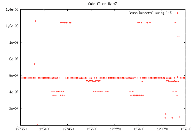
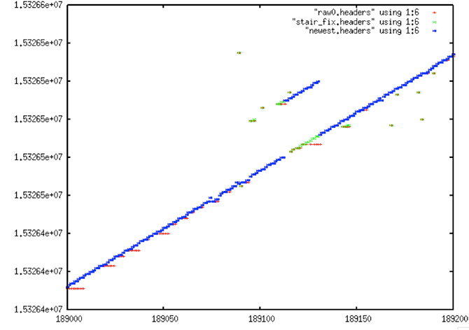
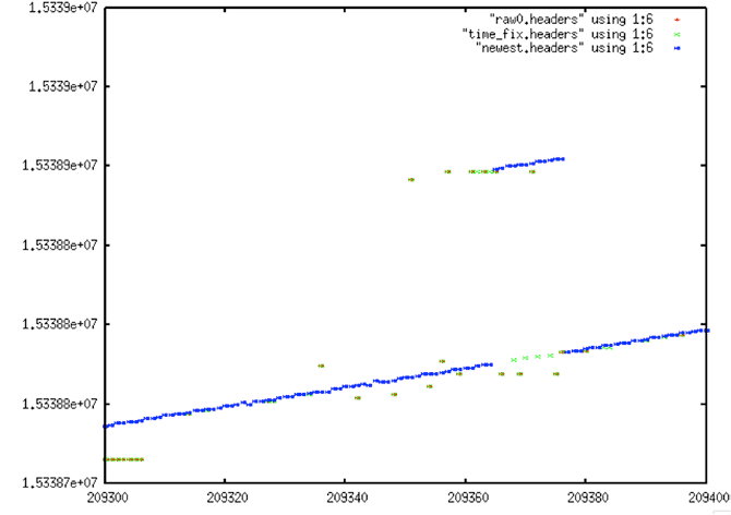
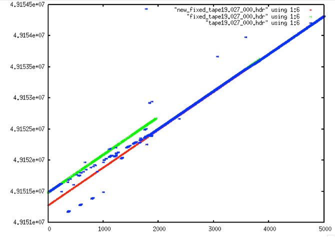
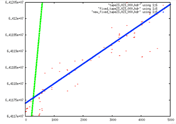
|---|
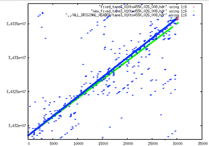
| Original Data |
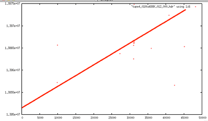 |
| Original Data: This example shows a dataset that is relatively clean before any filtering is applied. It seems that this file should have been extremely easy to clean. |
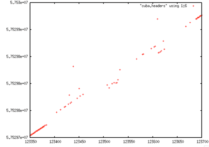
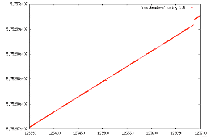
| Filtered Data |
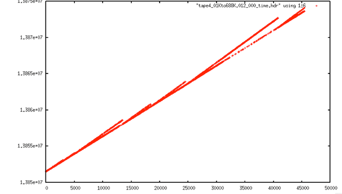 |
| Filtered Data: After the dataset went through the prep_raw.sh procedure, this was the resulting time plot. It is, quite obviously, very wrong. |
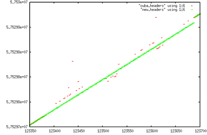
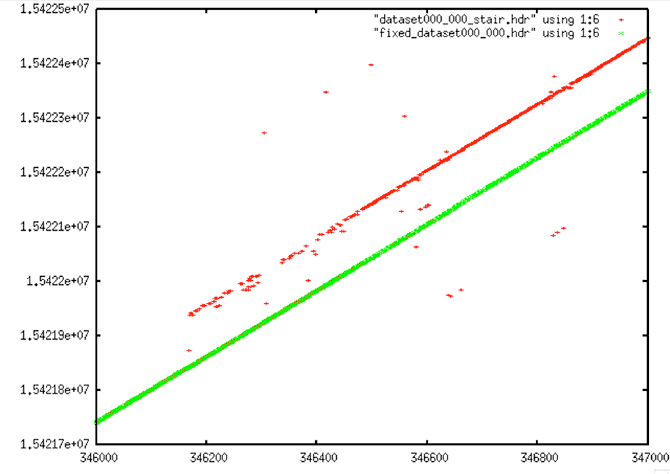
| Comparison |
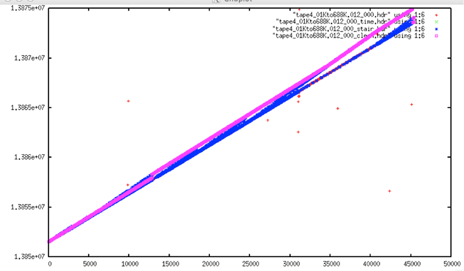 |
| Comparison of Original with Filtered: Although the times look fine in the first (unfiltered) plot, they are wrong for this satellite based upon the known PRI. The ASF cleaning software tried to fix these wrong time values using a known slope of 0.607. This introduced a discontinuity into the data and resulted in incorrect times. |
These results, wherein the time slope of the raw data does not match the known PRI of the satellite, were incredibly perplexing. At first, it was assumed that these data could not be processed reliably and were simply categorized into the large time-slope error and wrong-fix error categories.
Analysis of the time slopes in the original unfiltered data only pointed out how extreme the problem really was. Well over 100 files showed slopes that were either less than 0.606 or more than 0.608, with the lowest in the 0.48 range. The highest reliable estimate showed a slope of well over 0.62.
6.1 Slope Issues Explained
Eventually, through conversation with original Seasat engineers at the Jet Propulsion Lab (JPL), it was discovered that the Seasat metadata field MSEC of Day actually contains not only the time of imaging but also the time to transmit data from the spacecraft to the ground station. This adds a variable time offset to the metadata field. Once this was understood, it was readily obvious that using the known PRF as a guide for filtering was an incorrect solution.
Thus, the entire cleaning process was revisited, with all of the codes allowing more relaxed slope values during linear regression. This worked considerably better than the previous cleaning attempt. However, it did not solve the problems entirely.
6.2 Final Results of Data Cleaning
The final set of cleaned Seasat raw swaths was assembled using three main passes through the archives with different search parameters, along with a few files that were fixed on a case-by-case basis. Basically, the final version of the code was run and the results examined for remaining time gaps. Any files with large or many time gaps were reprocessed using different parameters. In the end, 1,346 swaths were cleaned, 2 by hand, 14 from the first pass, 25 from the second pass, and the remainder in the final cleaning pass. These then are the final cleaned Seasat archives for the initial release of ASF’s Seasat products.
| Date | Total Datasets | Dataset with Time Gaps | Largest Time Gap | Largest number of gaps in a file | Files with >10 msec gap |
|---|---|---|---|---|---|
| 1/31/2013 | 1,399 | 728 | 54260282 | 1820 | |
| 4/9/2013 | 1298 | 263 | 180 | 34 | |
| 4/9/2013 | 1,299 | 122 | 95 | 33 | |
| 4/9/2013 | 1,299 | 55 | 2113 | 17 | |
| 4/10/2013 | 1,299 | 34 | 50 | ||
| FINAL | 1,346 | 49 | 34 | 26 | 28 |
Final Cleaned Seasat Swaths: (table) Approximately one year after the project started, 1,346 raw Seasat swaths were cleaned and ready to be processed into SAR image products.
Written by Tom Logan, July 2013
Seasat – Technical Challenges – 7. Cleaned Swath Files
Seasat synthetic aperture radar (SAR) data holdings at ASF have been converted from their original 29 SONY SD1-1300L tapes into raw swath files with external metadata stored on disk. As detailed elsewhere in these pages, a total of 1,346 decoded, cleaned swath files were created.
The decoded data originally contained bit errors and discontinuities that had to be addressed prior to processing images. Cleaning the decoded data was an extensive process — critical metadata fields were median filtered to remove bit errors, time values were filtered into linear progressions, and discontinuities were filled with random values. In all, five separate filters were run on the telemetry data after it was decoded in order to prepare it for automated processing into image products.
The cleaned raw swath files come as file pairs. The unpacked raw data resides in a .dat file, and the decoded metadata resides in an .hdr file. The .dat files contain 13,680 byte samples of SAR data per line, so the file size for swath data files is always the number of lines in the file multiplied by 13,680 bytes.
The .hdr file contains a single entry for each line of data present in the corresponding .dat file. This entry is ASCII text formatted into 20 columns of integers recording the metadata decoded from the satellite time and status telemetry bits. If any discontinuities were found and repaired during the cleaning of the decoded data, then a third .dis file records the location and length of discontinuities.
Written by Tom Logan, July 2013
Seasat – Technical Challenges – 8. Focusing Challenges
In modern systems, synthetic aperture radar (SAR) echoes are sampled in a complex fashion using IQ-demodulation. The I and Q components are samples of the same signal that are taken 90 degrees out of phase. Separating I and Q in this way allows measurement of the relative phase of the components of the signal, and is a requirement for the SAR focusing algorithm. The Seasat platform used an older method to sample echoes, storing real (not complex) returns in offset video format.
The first step in processing Seasat SAR, then, is to be able to convert offset video into IQ format. Therefore, ASF selected the repeat orbit interferometry (ROI) package distributed by the Jet Propulsion Laboratory (JPL). ROI is a mature and robust SAR software correlator capable of processing offset video format signal data.
In order to focus Seasat SAR imagery using ROI, ASF created a configuration file using the cleaned header file and propagated state vectors. The decoding process created the cleaned header file. The propagated state vectors were obtained from NASA’s Goddard Space Flight Center. ASF chose to use ROI’s .in configuration file format. Initially this configuration file contained 47 parameters needed to create focused SAR data, but it was adapted to allow for up to 67 parameters to facilitate the removal of unwanted frequencies in the original signal data. (See “Range Spectra Filtering” for details).
Other technical challenges included propagating state vectors, Doppler estimation, overcoming Doppler ambiguities, filtering dirty range spectra, and creating proper data window position shift files to capture changes in the satellite’s delay-to-digitization metadata field.
Finally, using the decoded raw data, information from the decoded headers and propagated state vectors, proper configuration files were generated to allow ROI to focus the Seasat imagery.
8.1 Offset video format
A chirp signal has a symmetric frequency spectrum: the positive frequency band is symmetric to the negative frequency band about 0 frequency. To create a radio frequency signal, a chirp is mixed with a pure sinusoid at the desired radar frequency (L-band for Seasat), which then shifts the entire spectrum up to be centered around the L-band frequency with a side-band of frequencies on one side of the carrier and another side-band on the other side of the carrier.
These are all positive frequencies now, but two side-bands are created from the positive and negative portions of the original chirp spectrum. Offset video refers to the fact that the samples are real, not complex, so the spectrum contains both side-bands. The total bandwidth is in the “video” range (i.e. MHz), and the center of the bands are “offset” from 0 frequency so they don’t get mixed together. When the signal is converted from real samples to complex samples, one of the side-bands is saved, and the other one is thrown out. This creates what is called the “analytic signal,” which is complex.
It turned out that ROI, although programmed to process offset video SAR signal data, did not initially work correctly. The processor assumed the negative side-band was the correct one to use, but for Seasat the opposite side-band was required. Once this was discovered and a change was applied to ROI, the data focused properly. Many thanks to Paul Rosen of JPL for this discovery and for applying the fix that allowed the Seasat offset video format to properly focus in ROI.
Due to the nature of offset video format SAR data, the 13,680 original samples, once focused, only create half that number of range samples. Thus, focused Seasat imagery initially has 6,840 samples per range line (before further processing).
8.2 State Vectors
State vectors give the position and velocity of a satellite at a given time. ASF compared state vectors derived from Two Line Element files at CelesTrak with the Seasat precise orbits solutions made as part of NASA’s Ocean Altimeter Pathfinder Project . It was determined that the precise orbit solutions gave better geolocations in final products and were, therefore, used in the production of the Seasat detected image archives.
Although state vector creation and propagation is a fairly routine task within satellite processing systems, a non-standard transformation was required in this project. Since ROI expects the state vectors in platform-centered velocity and acceleration coordinates, the conversion code from ROI_PAC was utilized to create the final state vectors inserted into the ROI configuration file.
8.3 Doppler Centroid Estimation
The Doppler centroid locates the azimuth signal energy in the azimuth (Doppler) frequency domain, and is required so that the azimuth compression filter can correctly capture all of the signal energy in the Doppler spectrum, thereby providing the best signal-to-noise ratio and azimuth resolution. Thus, even with good knowledge of the satellite position and velocity, a Doppler centroid frequency must be accurately estimated in order to focus SAR data.
The Doppler centroid varies with both range and azimuth. The variation with range depends on the particular satellite attitude and how closely the illuminated footprint on the ground follows an iso-Doppler line, as a function of range. The variation in azimuth is due to relatively slow changes in satellite attitude as a function of time. Because the change is slow, the azimuth Doppler variation is minimal within a single Seasat frame and so was ignored.
The azimuth signal in SAR is sampled by the pulse repetition frequency (PRF). As with all sampled signals, there is an ambiguity in the location of frequency spectrum, by a multiple of the sampling rate. For this reason, the Doppler centroid is written as:
fr = fr’ + M*PRF
Here, the absolute Doppler frequency at range sample r, fr, is composed of two parts. The fine Doppler centroid frequency fr’ comprises the fractional part, and is ambiguous to within the azimuth sampling rate, which is the PRF. The other part is an integer multiple of the azimuth sampling rate M*PRF. Doppler centroid estimation often refers to the estimation of the fine Doppler centroid frequency, which is limited to the range ± PRF/2. The Doppler ambiguity M is an integer in the set {-2, -1, 0, 1, 2}. The two components of the unambiguous Doppler centroid frequency, fr’ and M, are estimated independently.
Because of the range-variation of the Doppler centroid, the Doppler centroid is estimated at different ranges in the data, and a polynomial function of range is fit to the measurements.
ROI expects the three coefficients for a quadratic equation whereby the Doppler centroid at a given sample can be calculated as a percentage of the PRF. Fortunately, the fractional part, fr’, can be determined directly from the signal data using a fairly simple technique known as pulse-pair Doppler centroid estimation.
Given: A, B, PROD and DOP all arrays of length 16K
Start at middle of file – 5000 lines, continuing for 10000 lines
A = convert offset video at line X to I,Q by forward/reverse FFT
B = convert offset video at line X+1 to I,Q by forward/reverse FFT
PROD +=sum(conj(A)*B)
DOP=-1.0 * ATAN2(PROD.IMAG,PROD.REAL)/2π
Pulse-Pair Doppler Centroid Estimation: Calculate the complex conjugate of line X times line X+1. Sum these products for 10,000 lines. The Doppler centroid is then estimated for each range sample by calculating the resultant phase of the product using the ATAN2 function.
Unfortunately, this only determines the fractional part of the Doppler centroid; the result is always ±50 percent of the PRF (i.e. from -823 Hz to +823 Hz). In some cases, Doppler values as high as 2000 Hz or as low as -2000 Hz were observed in the Seasat data. Thus, a Doppler of 0.3 PRF could be -1153 Hz, +494 Hz or even as much as +2141 Hz based upon the value of the Doppler ambiguity M. So, even with the pulse-pair Doppler centroid estimation algorithm, additional processing was required to determine the proper Doppler ambiguity.
Also, for much of the Seasat mission, a calibration pulse was embedded in the transmitted signals. This has the effect of invalidating the Doppler centroid estimate in the center of the imaging swath as well as introducing a solid white line down every focused product created from such data.
So, to estimate the range-dependent Doppler centroid, ASF used an altered pulse-pair algorithm, first modified to ignore the values estimated in samples 3180 – 3980. Next, a wrap-around ambiguity resolution was applied and finally, a small set of heuristics were applied to the Doppler constant to try to guess the correct Doppler ambiguity for each scene based upon the satellite direction of travel (ascending or descending) and position (higher or lower latitude).
Still, since only 94 percent of scenes automatically focused, each image had to be examined by a man-in-the-loop quality control procedure, not only for focusing problems, but also for the remaining data quality issues discussed in “Remaining Data Quality Issues.”
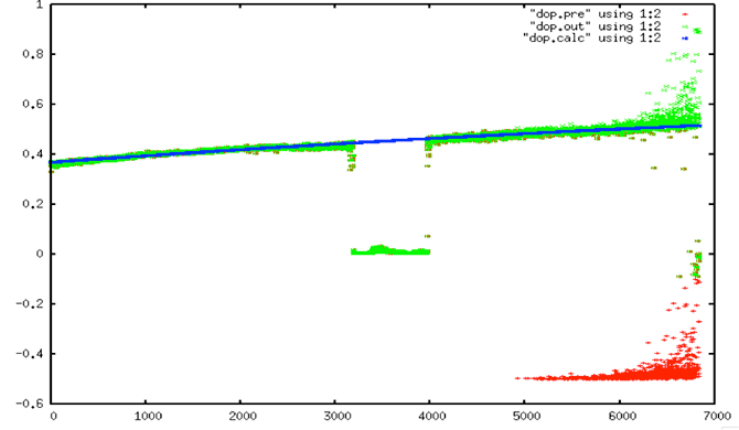
Doppler Estimation: In this plot, the Doppler centroid estimate as a percentage of the PRF (Y-axis) is plotted against range samples (X-axis). The red plot is the original estimate, and shows the wrap-around in the bottom right side of the figure. The green plot has fixed the Doppler wrap-around ambiguity. The blue line shows the quadratic fit that was finally used. Note that the calibration pulse invalidates samples 3180 – 3980, always showing a near-zero Doppler value.
8.4 Range Spectra Filtering
A power spectrum describes how the power of a signal or time series is distributed over different frequencies Because SAR uses a linear FM chirp, the power should always be distributed evenly in an image’s spectra. Because SAR data has distinctive range spectra, one method to check whether signals are valid SAR data is to plot the power spectra.
This was done early in data exploration, showing additional problems with the Seasat raw signal data. Rather than show the standard relatively flat peak, the Seasat spectra show tones that should not be present in raw data.

Seasat Range Spectrum: This plot shows the power spectrum of Seasat signal data plotted as a function of the range frequency bin. Although the DC Bias at bin zero is expected, the additional tones make this a “dirty” spectrum. The largest tone always appears at +/- fs/4, while the other spurious tones appear in a variety of frequency locations. [Figure created by Paul Rosen, JPL].
Fortunately, ROI has a built-in feature for the removal of specific frequencies that were inserted into the signal data for calibration purposes. These frequencies are called “caltones,” or calibration tones. The feature in ROI works as a notch filter, and ASF was able to modify it to remove up to 20 unwanted caltones. To determine the frequencies to remove, the steps outlined in the Spectral Filtering Algorithm were taken.
- Calculate the range power spectra
- Calculate the mean and standard deviation of the spectra
- Sort all spectral values that are greater than 1.5 standard deviations from the mean into descending order
- Cull the list to remove neighboring caltones: All tones within 6 bins of a tone previously in the list are removed. This ensures only a single frequency will be removed in given neighborhood of bins.
- Remove up to the top 20 values left in the list
Spectra Filtering Algorithm: All values greater than 1.5 standard deviations from the mean spectral value are gathered and sorted. Closely neighboring caltones are culled, creating the final list of caltones to be removed via notch filtering.
Once the power spectra have been filtered to remove these caltones, many artifacts are removed from the Seasat images.
| Range Spectra Filtering |
|---|
| Unfiltered Spectra |
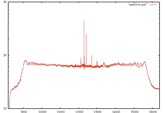 |
| Unfiltered Spectra: A Seasat range power spectra showing spurious tones to be removed. This plot shows the power spectrum of Seasat signal data plotted as a function of the range bin. It only shows the upper complex spectrum, not the conjugate. |
| Representation of the Filtered Spectra |
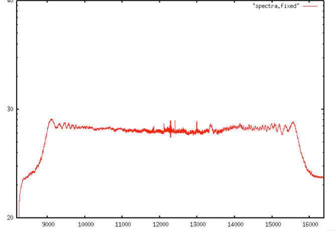 |
| Representation of the Filtered Spectra: After filtering, the range spectra have outlying peaks removed. This plot shows the power spectrum of Seasat signal data plotted as a function of the range bin. It only shows the upper complex spectrum, not the conjugate. |
| Unfiltered Spectra |
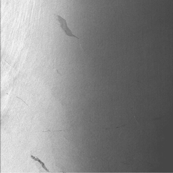 |
| Unfiltered Spectra: This version of Seasat product SS_00472_STD_F3099 was focused without the removal of caltones. Vertical lines are visible in the far range. |
| Filtered Spectra |
|
| Filtered Spectra: Once the spurious caltones were removed using a notch filter, the vertical lines disappeared. Tones at 0.25, 0.25885009765625, 0.29449462890625 and 0.29339599609375 were removed. |
| Unfiltered Spectra |
|
| Unfiltered Spectra: Product SS_01385_STD_F1145 processed without caltone removal shows many vertical lines in the far range. |
| Filtered Spectra |
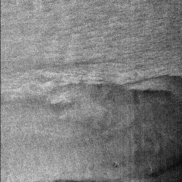 |
| Filtered Spectra: Once the caltones are removed (13 in this case), many of the vertical lines are gone. Unfortunately, this method is not perfect, and some lines are still visible in the image. |
8.5 Data Window Position Shifts
The time delay between transmitting a SAR pulse and receiving an echo is directly related to the altitude of the satellite at the time of imaging. Based upon changes in orbital altitude, this delay may change a handful of times in any given datatake. As the satellite altitude changes during an orbit, the change is quantified using the delay-to-digitization field. During focusing, the slant range to the first pixel is calculated using these quantified values.
Prior to the application of the delay-to-digitization parameter in the ASF Seasat Processing System (ASPS), cross-track ghosting was readily observed in images that contained delay shifts. This was addressed using another one of ROI’s built in features – the data window position (DWP) file.
This file contains one entry for each delay-to-digitization shift found in a swath. Each such entry contains a <line, value> pair where line is the line number in the cleaned raw swath data to apply the shift and value is the amount of the shift. This DWP file is then passed to ROI where the DWP shift is implemented.
| Data Window Position Shifts |
|---|
| Cross-Track Ghosting |
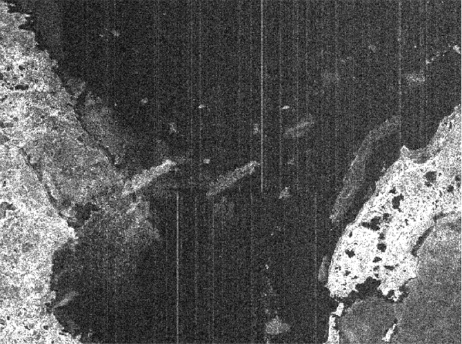 |
| Cross-Track Ghosting: This processed image did not have a valid DWP file for ROI. An across-track ghost of the island near the left of the image can be seen. Also, the vertical lines (resulting from noisy signal data) do not line up from top to bottom of the image. |
| Ghosting Removed |
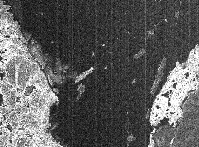 |
| Ghosting Removed: Once a valid DWP shift file was created and made available to ROI, the cross-track ghosting was removed from the image. Also note how the vertical lines (resulting from noisy signal data) now match from top to bottom of the image. |
Written by Tom Logan, July 2013
Seasat – Technical Challenges – 9. From Swaths to Products
At this stage in the development of the ASF Seasat Processing System (ASPS):
- 1,346 cleaned raw signal swaths were created
- Repeat Orbit Interferometry (ROI) was modified to handle Seasat offset video format
- New state vectors were selected for use over two-line elements (TLE’s)
- Caltones were filtered from the range power spectra
- Data window position files were created
- The remaining tasks before wholesale image creation could begin were (1) automated creation of the ROI input files with all fields properly filled and (2)
- implementation of a product framing scheme.
9.1 Creation of ROI Configuration Files
The program create_roi_in was developed for the purpose of gathering all of the information necessary to focus a particular piece of Seasat data into complex imagery.
create_roi_in:
- Using the .hdr file of metadata
- Determine exact start, center and end time of signal data section to be focused
- Find any changes in the delay-to-digitization in this section of signal data
- Create a DWP file if necessary, marking all shifts that occurred
- Use the minimum DWP to calculate the slant range to first pixel
- Propagate the state vectors to the exact middle time of the scene and convert into ROI’s internal format for the spacecraft height, velocity and acceleration
- Estimate the Doppler centroid using filtering and regression to get a quadratic fit
- Calculate the range spectra, filter and get galtones to be removed
- Write all values to the .roi.in file
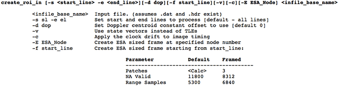
ROI Configuration File Creation Program: Many command line options are offered by create_roi_in, including the ability to process any amount of signal data or the exact amount of signal data needed to create a single 100-km2 image framed by European Space Agency (ESA) framing standards.
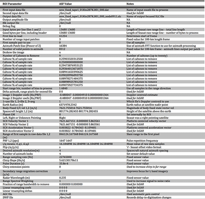
Modified ROI Configuration File: The ROI .in configuration file used to process image SS_00638_STD_F0911. ASF ROI configuration files allow for up to 67 lines of parameters to be passed. Note that ROI is the Repeat Orbit Interferometry correlator, and as such it is set up to process InSAR pairs of imagery. When utilized for processing single Seasat images, many ROI parameters are either not applicable or simply repeated (as in the case of input bytes per line, good bytes per line, spacecraft velocity, PRF, etc.). Most parameters are fixed based upon the sensor being focused. However, some parameters vary in each scene since they are either data dependent (i/q mean, caltones to remove, Doppler centroid) or platform-location specific (body fixed velocity, earth radius, spacecraft altitude, velocity and acceleration, range of first sample).
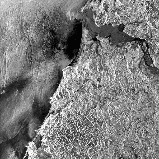
SS_00638_STD_F0911: Seasat image created using the parameters in the modified ROI configuration file.
9.2 Framing Data Products
ASF divides swaths of SAR data into individual frames that are bundled into products and made available for download. Seasat swaths are divided into 100-km2 scenes centered at European Space Agency (ESA) standard nodes. The naming convention for Seasat products is as follows:
SS_00000_STD_Fffff
Where 00000 is the five-digit orbit number of Seasat platform at time of imaging and ffff is the four-digit ESA node number signifying the center latitude of the product.
9.2.1 Modified ESA Frames – Product Length Determination
ASF elected to use the ESA node scheme as it is common to other products and understood by many SAR researchers. From “ESA EOHelp Frequently Asked Questions”:
The European Remote-Sensing Satellite (ERS) orbit is split into 7200 nodes and 400 are used to identify the SAR frames through the node closest to the frames’ center. Therefore, the identifiers of two adjacent frames differ by 18 nodes. The first frame starts at the equator and is identified by node 9, the last one by number 7191.
The frames between number 9 to 1791 and 5409 to 7191 are in the ascending part of the orbit.
A satellite orbit is split into two parts:
- the ascending pass
- the descending pass
The ERS-1 satellite has the following scheme:
Equator North Pole Equator South Pole Equator
9 1800 3609 5400 7191
|—ascending—|————–descending———–|—ascending—|
where the numbers are standard frame numbers
When the scheme above was implemented using frames centered 18 nodes apart, large gaps existed between the framed Seasat products. This can be explained as follows: splitting the earth up into 7,200 nodes means that each node is 0.05 degrees of latitude. If images are framed 18 nodes apart, then the centers are 18 * 0.05 degrees = 0.9 degrees of latitude apart. A degree of latitude varies from 110.6 km to 111.7 km from the equator to the North Pole. Therefore, 0.9 degrees of latitude varies from 99.54 km to 100.53 km from the equator to the North Pole.
It follows that even if the orbit of Seasat was directly north-south, little to no overlap could be expected for 100-km length scenes. However, Seasat had an orbital inclination of 108 degrees, a full 10 degrees further off vertical than ERS-1, the satellite for which ESA designed these nodes. Thus, Seasat covered considerably less latitude per 100 km of travel than the ERS satellites.
Nodes 0 – 1800: center latitude = node*.05
Nodes 1801 – 3600: center latitude = 180.0-(node*0.05)
ESA Frame Center Calculations: Nodes 0 – 1800 are ascending in the Northern hemisphere. Nodes 1801 – 3600 are descending the Northern hemisphere. Nodes 3601 – 7200 are located in the Southern Hemisphere, so they will never be used for the Seasat data collection.
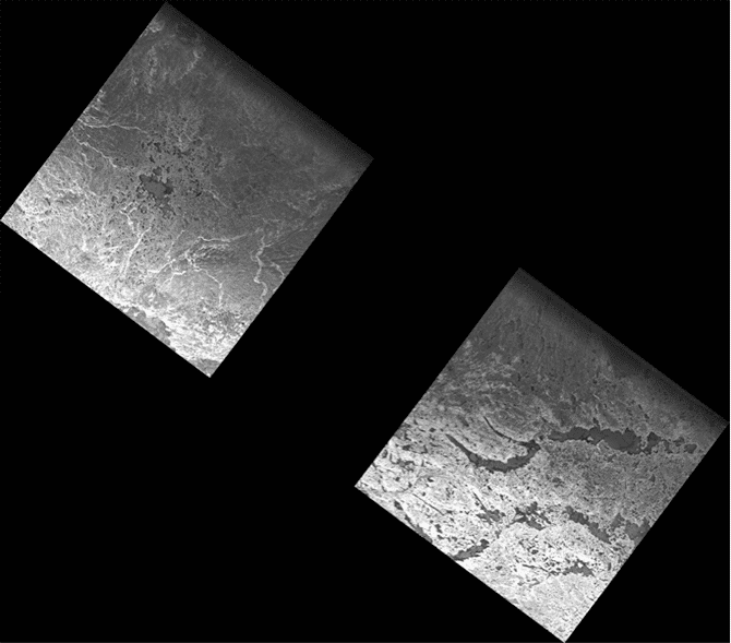
Using ESA Standard Frames: These images were framed using the standard ESA framing technique (frame 78 and 79) and then mosaicked to check for overlap. Since there is black between the images, the standard ESA framing schema is not valid for Seasat products.
Due to differences between the ERS-1 and Seasat orbits, a modified ESA scheme was implemented for Seasat products. At first, the number of nodes between framed centers was simply halved, i.e. products were created with centers only nine ESA nodes apart.
This scheme worked until the higher latitudes, where the satellite’s orbital path goes from ascending to descending. At this part of the orbit, the satellite actually stops ascending in latitude and starts descending. In this case, 100 km of satellite motion is considerably less than nine nodes of latitude change. Thus gaps once again existed between framed products.
Finally, then, the ASF Seasat SAR framing scheme allows a variable number of ESA nodes to pass between frames. Each frame is 100 km in length and centered at the ESA node that gives roughly 15 percent overlap with the adjacent frames. Thus all Seasat products are the same size but spaced variably along-track. Since Seasat only imaged in the Northern hemisphere, only ESA nodes 0 – 3600 are ever used.
| Modified ESA Frames |
|---|
 |
| Modified ESA Frames: This mosaic shows two Seasat products created nine ESA nodes apart (1278 – 1287). In this case, the mosaic shows no gap exists between these framed products. |
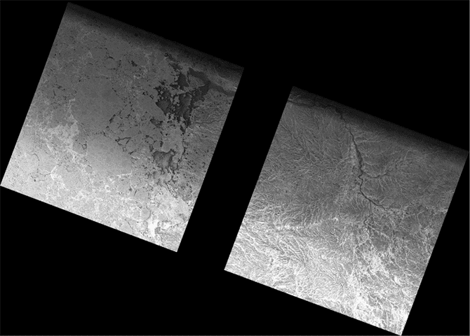 |
| Modified ESA Frames: This mosaic also shows two Seasat products created nine ESA nodes apart (1467 – 1476). However, because these images are at a higher latitude, there is a gap between processed frames. The nine-nodes-between-centers method did not work properly for Seasat. |
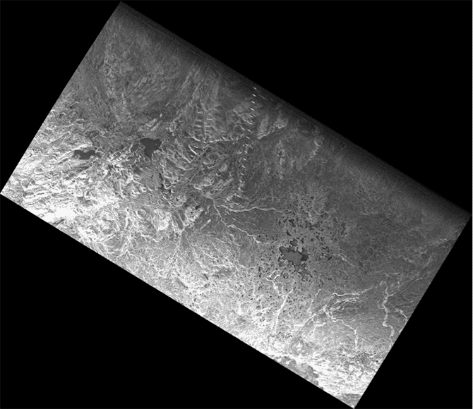 |
| Framed Seasat Product Mosaic: Mosaic of two Seasat framed products showing how the modified schema with variable nodes between centers ensures overlap between framed products. |
Aside: Example of Products Created from a Single Cleaned Swath – Processing cleaned swath file new_fixed_tape4_01Kto688K.001_000.dat resulted in the following list of products (ESA node numbers highlighted in blue):
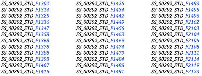
Note that orbit number 00292 goes from ascending (nodes 1302 – 1496) to descending (2102 – 2123). Note too how the ESA node numbers get closer together as the satellite approaches the northern tip of its orbit. The same applies in reverse on the descending part of the orbit: At first images are centered just one ESA node apart, but the number of nodes between frame centers grows as the satellite continues south.
9.2.2 Far Range Samples – Product Width Determination
SAR processing is performed on specifically sized pieces of signal data called patches. Patches are generally an even power of 2 in size to facilitate the FFTs that are used during focusing. Range patches are in the range direction; for Seasat only a single range patch of length 8192 is needed to process the entire range direction of 6,840 samples. Azimuth patches are in the azimuth direction. Azimuth patches can vary in length. For Seasat a length of 16,384 (16K) was used.
The SAR processing algorithm requires a certain amount of overhead per range patch and azimuth patch processed. This overhead is either the length of the azimuth reference function for the azimuth direction or the range reference function for the range direction. The length of these functions determines how many samples are combined to make a single return in the focused image. For Seasat, the range reference function is always 1,539 samples, while the azimuth reference function varies in length from around 5,500 to as much as 5,700.
Dealing with the overhead in the azimuth patches is straightforward. For each azimuth patch, process 16K lines of data and only keep 16K minus the patch overhead lines. Seasat processing only utilizes 8,312 lines per azimuth patch, well under the number of valid lines actually created.
The range reference function overhead is more difficult to deal with. All of the literature states that Seasat boasts a 100-km width swath. However, of the 6,840 range samples that can be created per line, only 5,301 samples are known to be valid (5,301 = 6,840 range samples minus the 1,539 overhead). When these samples are mapped from natural slant range spacing into 12.5-meter ground range spacing, 7,166 valid range samples are created. This means that the actual valid width of the Seasat swath is
7,166 samples * 12.5 meters/sample = 89,575 meters,
considerably less than the 100 km advertised.
Thus, it had to be determined if Seasat products should be 100 km 2, even if it meant keeping some partially valid samples in the far range, or should products be less than 100 km 2 , keeping only known valid pixels. The decision was made to create 100-km wide swaths even though this may introduce a few pixels in the far range that do not contain the contributions from a full 1,539 raw samples. As a result, users may notice slight darkening in the last 824 range samples in some images. This is intentionally done in order to create square Seasat products.
9.3 Data Quality Tool
Due to Doppler ambiguities that could not be automatically overcome, each Seasat product created at ASF is examined using a specially designed quality control tool. This QC tool allows each product to be visually inspected and accepted, reprocessed, or discarded. If a product is not focused, it is reprocessed at the next logical Doppler ambiguity. If a product contains less than 50% valid data it is discarded. Finally, if a product is accepted, an annotation file is made providing an indication of data quality issues observed in the product. Each of these remaining data quality issues will be discussed in “Quality Issues.”
9.4 Processing Results
Once the programs that create a single image product were developed and tested, they were all encapsulated in a main program referred to as create_base_images. Given an input cleaned swath file, create_base_images creates all framed products covered by a datatake. Each swath is run through this procedure in order to create the beta set of framed Seasat images and corresponding metadata.
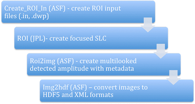
Single Image Processing Flow: In order to create an individual framed product, a cleaned swath file goes through (1) creation of the configuration file(s) for ROI, (2) focusing into SLC imagery using ROI, (3) creation of multilooked amplitude images, and (4) conversion of images into HDF5 with ISO compliant XML metadata.
Each of these images are visually examined using the ASF Seasat Quality Control Tool, which allows one of three actions to be taken:
- Images that show less than half a frame of valid SAR data are discarded.
- Images that are not properly focused are sent through a reprocessing step, which modifies the Doppler constant in order to determine a Doppler centroid that will focus the product.
- Images that are properly focused and contain more than 50 percent valid SAR data are added the to the ASF data pool. Each product also contains an annotation file to inform the end user of any quality issues encountered during the visual QC check.
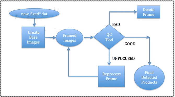
ASF Seasat Processing System (ASPS) V1.0: All cleaned decoded swaths were passed through the create_base_images procedure, which created the framed product files. Due to Doppler ambiguities and data quality issues, each product had to be examined using the QC Tool, which took one of three actions: (1) If the image is good, publish it; (2) If it is unfocused, reprocess it at a new Doppler; (3) If the image is not valid SAR data, delete the product.
Written by Tom Logan, July 2013
Seasat – Technical Challenges – 10. Quality Issues
After the decoding, cleaning and focusing of the Seasat synthetic aperture radar (SAR) data, many artifacts still exist in the initial ASF Seasat SAR products. Most of the artifacts observed in the images result from system interferences during data acquisition, missing data as a result of multiple transcriptions between media storage since 1978, and processing decisions implemented in the ASF Seasat Processing System. ASF’s intent is to distribute as much of the historic dataset as possible to our users while offering transparency about known quality issues.
These anomalies can be split into those known to be caused by the sensor and those that are visible in the imagery but not tied to a specific cause.
10.1 Sensor Anomalies
Some anomalies in the ASF Seasat products have a known cause, originating in some fashion from the platform itself. Sections of no valid data occurring at the beginning and end of many swaths result in frames with missing imagery. A calibration pulse embedded into some of the signal data appears as a bright line in the center of focused frames. An additional calibration signal manifests as a pattern of dashed lines. Finally, some images show extreme attenuation due to incorrect sensor parameters.
10.1.1 No Data
During processing, several swaths showed no data at all. Most likely the satellite was in a test mode during these times. These products were discarded. However, many of the original swaths start with no data being collected, introduce real data after some number of lines and end the datatake with another patch of no data collection. This means that swaths contain both invalid and valid data. Since the bit fields that may have given information on whether the satellite was actually imaging were unreliable, ASF chose to process all of the data in each swath.
Then, during the Quality Control (QC) process, products that contained less than 50 percent valid SAR data were discarded. Products that contained more than 50 percent were kept and made available in the ASF data pool. Thus, some of the ASF Seasat products contain areas of no valid SAR data, which are easily identified by blackness resulting from having no data to focus during processing.
| No Data Examples |
|---|
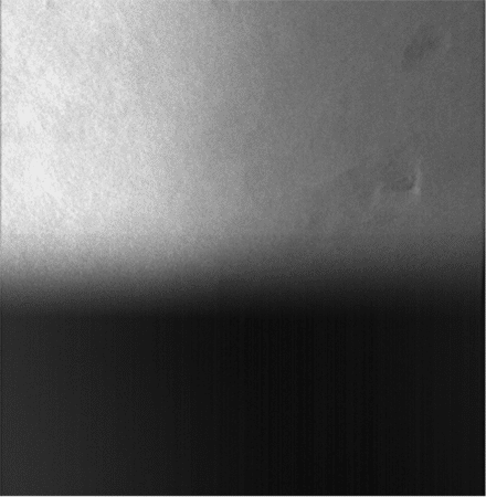 |
| No Data: The bottom half of this scene holds no valid SAR data. It was decided that any scene with more than 50 percent valid data would be saved and published. |
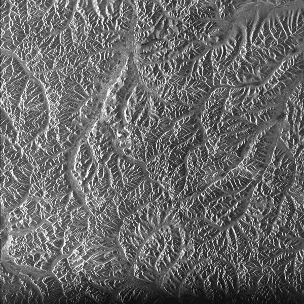 |
| No Data: This scene ran out of valid data right at the end of focusing. Note how the brightness fades as each successive line has less and less valid data to focus. |
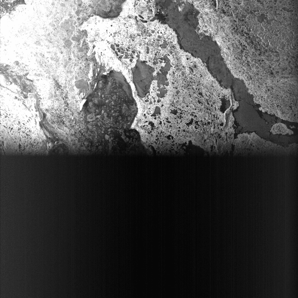 |
| No Data: This image has no valid SAR data in the bottom half. |
10.1.2 Calibration Pulse
During the start of the Seasat mission, when engineers were still testing system parameters, a calibration pulse was introduced into the raw signal data. Unfortunately, because the mission was cut so short by a power failure, much of the Seasat data has an embedded calibration pulse.
This pulse, when focused, forms a bright white line in the azimuth direction, somewhere near the middle of the swath.
Initial investigations into the calibration pulse show that it can be removed algorithmically. It is ASF’s intention to remove the pulse in future releases of Seasat SAR products.
| Calibration Pulse Examples |
|---|
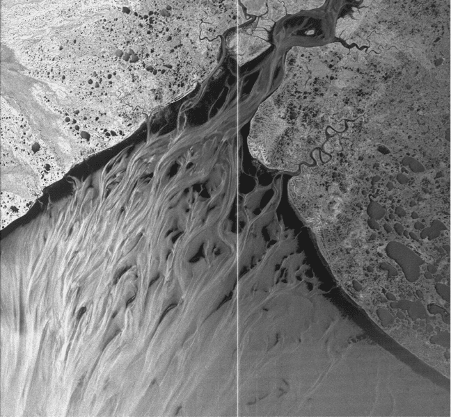 |
| Calibration Pulse: Kuskokwim Delta, Alaska — This image shows the effects of the calibration pulse — a white line in the azimuth direction near the middle range of the image. Also visible is banding near the bottom of the image. |
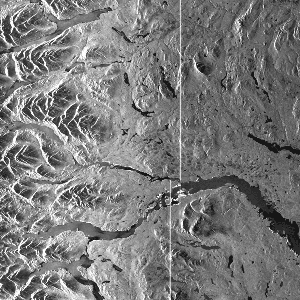 |
| Calibration Pulse: This image again shows the calibration pulse line near the middle of the image. Also readily visible is the effect of a data window position shift on the calibration pulse’s location in the image. |
10.1.3 Dashes
Another signal was embedded into the Seasat raw data. This one creates a set of short lines across the range direction of an image when focused. It has been verified that this signal is a real occurrence in the raw data. It is not known what the origin or intent of this signal was. It is noted that whenever this signal is present in the data, the calibration pulse is not.
Although often the calibration pulse precedes and follows a section of dashes in an image, it also appears in data that has no calibration pulse. It is unclear if this signal can be removed from the raw data in a future release of ASF Seasat products, but that step will be examined for feasibility.
| Dashes Examples |
|---|
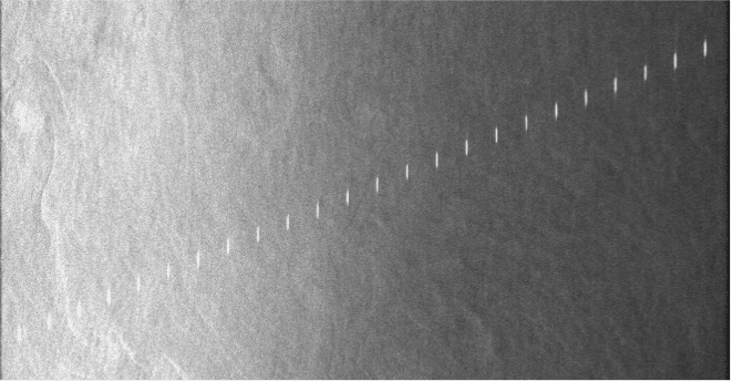 |
| Dashes: A distinctive pattern of lines occurs regularly in focused Seasat data. |
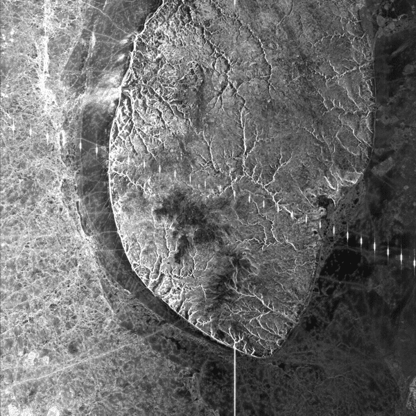 |
| Dashes: The dash pattern across this image occurs in several Seasat images. It is noted that the whenever the dashes occur, the calibration pulse stops. This indicates that the dashes were intentionally placed into the signal data by Seasat engineers. |
10.1.4 Attenuation
Some of the ASF Seasat products have extreme across-track attenuation. The effect is that the near range of the image is very bright, while the far range is quite dark. It was initially thought this had to do with the gain control on the satellite (which was one of those unreliable bit fields). However Jet Propulsion Lab (JPL) engineers indicate that it is possible this was caused by incorrect delay-to-digitization settings during the first part of the Seasat mission. In any case, this effect probably can never be removed from the imagery, only noted as a data quality issue.
| Attenuation Examples |
|---|
| Extreme Attenuation |
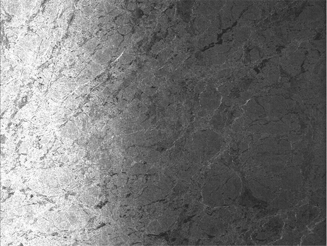 |
| Extreme Attenuation: This image shows the extreme attenuation present in some of the Seasat imagery. It is understood that this resulted from an incorrect parameter setting. |
| Not Extreme Attenuation |
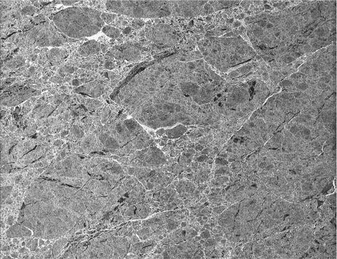 |
| Not Extreme Attenuation: For comparison purposes, here is another Seasat image that shows similar content (sea ice) but does not display the extreme across-track attenuation. |
10.2 Image Anomalies
It is commonly known that SAR imagery often has data anomalies, arising during image acquisition or processing, that visually impact focused products. These can be the result of atmospheric effects or of missing data. It is possible they are effects from the data cleaning not being done properly. In time, the causes for many of these anomalies may be determined and addressed; however, ASF has not yet completed a full analysis. Still, the following anomalies were noticed and annotated during the visual QC process.
10.2.1 Banding
Banding across SAR imagery is a fairly common occurrence and can be the result of atmospheric effects or poor data. Some banding was noticed in the ASF Seasat products.
| Banding Examples |
|---|
 |
| Across-Track Banding: Often very subtle, across-track banding like that visible in this image occurs in some of the Seasat SAR products created at ASF. |
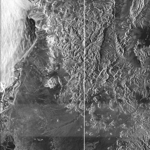 |
| Across-Track Banding: In this example, only a single band is present across the bottom of the image, but it is quite bright. |
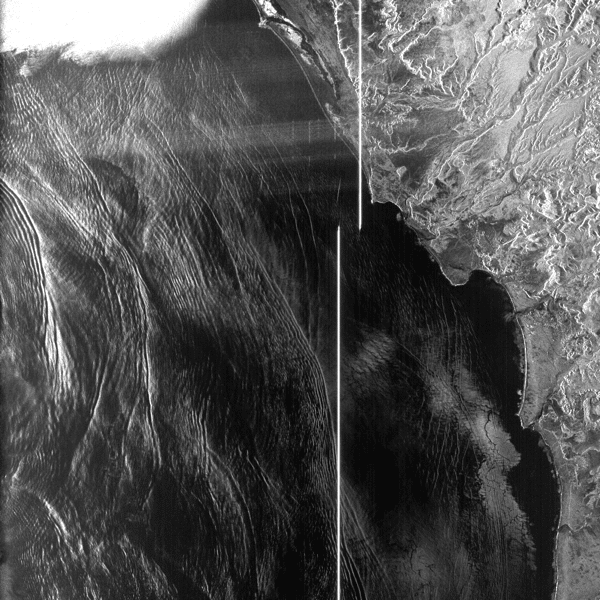 |
| Non-regular Banding: It is common for across-track banding to show some curvature, as is displayed across the top of this image. This is due to the range migration portion of SAR focusing. |
10.2.2 Along-Track Streaks
Much, if not all, of the Seasat imagery shows some amount of along-track streaking. Although ASF removed some of these streaks using the range spectra filtering, some remain.
| Along-Track Streaks Examples |
|---|
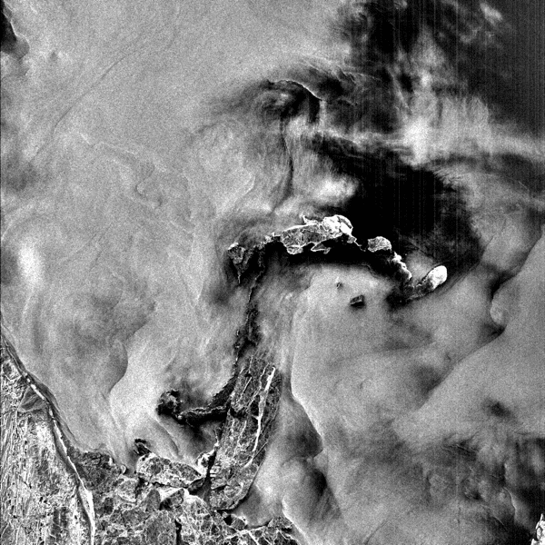 |
| Along-Track Streaks: In spite of the spectral filtering applied, some Seasat imagery still displays along-track streaks. Since these occur in much of the imagery, they are most likely due to systematic sensor or data collection errors. The cause is being investigated. |
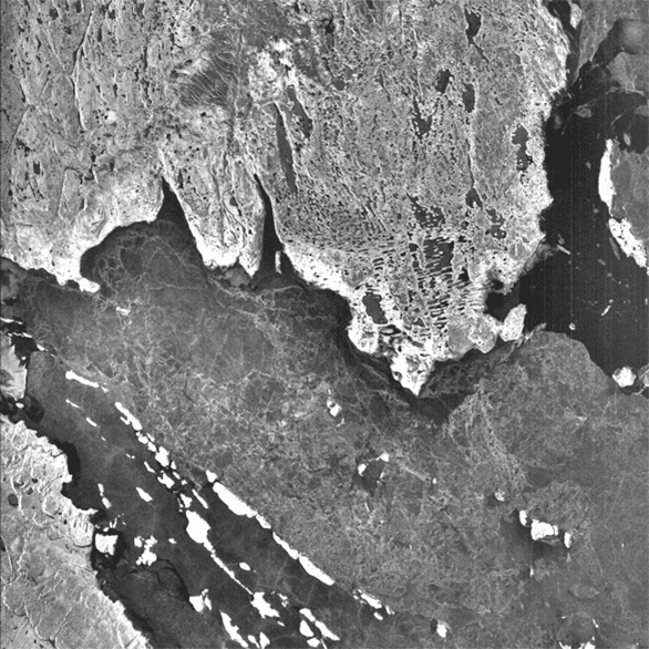 |
| Hidden Streaks: Often along-track streaking is hidden by brighter returns in the imagery. However, when dark areas occur, especially in the far range, along streaks become obvious. |
10.2.3 Across-Track Streaks
In addition to the along-track streaks, across-track streaks also occur. Typically these are lines across the imagery, often bent in one direction or another. This bending results from the range migration portion of the SAR focusing algorithm.
| Across-Track Streaks Examples |
|---|
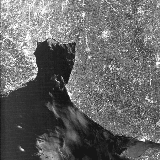 |
| Across-Track Streaks: Across-track streaking is readily obvious in this scene. |
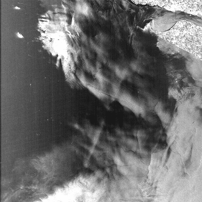 |
| Along-Track and Across-Track Streaks: Some imagery evidences multiple data quality anomalies, like this image with both across-track and along-track streaks. |
10.3 Missing and Partial Lines
When the Seasat data was first decoded, over half of the datasets showed time gaps. In the end, missing lines were filled with random values in 494 out of 1,346 swath files. Although the worst saved file had 136 gaps filled, only 34 files had 10 or more gaps, while 288 files had only one or two gaps in them.
To ensure users are fully aware of data anomalies that may cause analysis issues, any missing lines that occur within the raw data used to focus a product are annotated in the XML metadata files provided with the products.
Data Gap Information in XML: Each time a data gap occurs in the raw data used to create an ASF Seasat product, it is annotated inside the XML metadata file.
In addition to missing lines, partial lines occurred regularly during the Seasat decoding. In fact, some number of partial lines were found in 1,170 of the 1,346 cleaned swath files processed at ASF. The worst files had up to 42 percent partial lines. However, those files did not process correctly. Only files with less than 4.5 percent partial lines focused into imagery. Only 32 of the cleaned swath files that ASF processed into products had more than 1 percent partial lines.
Several of the swaths with the worst partial lines were processed and examined visually for effects; none were noticed. It was noticed that in most cases the majority of partial lines occurred near the start of the first product in a swath. This makes sense, as SyncPrep broke raw signal files into pieces when the data was first byte-aligned. SyncPrep breaks the files only if it loses sync, i.e. if a bad section of data is encountered. It is no wonder then that the start of many of these swath files have some amount of partial data in them.
Because of the lack of visual effects from the partial lines and the small number of files affected by any large amount of partial data, this information was not annotated in the metadata files. It is possible that in future releases this information may be made available in the product metadata if it is requested.
10.4 Missing and Partial Lines
In the beta release of ASF Seasat products, no advanced geolocation corrections were applied. However, a few modifications were made during development that have brought the observed geolocation errors to within 1 kilometer in most cases.
ASF compared state vectors derived from Two Line Element files at CelesTrak with the Seasat precise orbits solutions made as part of the NASA Ocean Altimeter Pathfinder Project. It was determined that the precise orbit solutions gave better geolocations in final products and were, therefore, used in the production of the Seasat detected image archives.
Satellite imaging times were filtered as accurately as possible. First, a crude time filtering was applied to fix gross errors greater than 513 from the local trend line. Next, sticking satellite clock times were brought into line, and a final linear fit was performed to bring all time values to within 2 msec of the new linear trend. Then, all discontinuities in the time fields of the data were found and fixed. Finally, the start times of all files were changed to match the linear trend of the rest of the file.
Although ASF has not undertaken a thorough analysis of geolocation accuracies, it was noted that Seasat geolocations usually show an across-track error. To adjust for this, a negative 1,000-meter slant range shift was introduced into the products when calculating georeferencing information. Users are advised that when attempting to recreate the geolocations stored in either the HDF5 or the GeoTIFF products, this -1,000-meter slant range shift must be taken into account.
In the end, the data quality group at ASF examined only six different sites for geolocation accuracy. Each image’s geolocations were matched against the same feature in an Advanced Land Observing Satellite (ALOS) Phased Array L-band Synthetic Aperture Radar (PALSAR) image. This removed any concern over geolocation shifts dues to terrain height; i.e., the terrain height would affect both the Seasat and the ALOS images similarly, meaning the effect would be cancelled out.
| Site Location | Observed Geolocation Offset |
|---|---|
| Albany, OR | 1300.7 |
| Big Delta, AK | 908.8 |
| Datchet, England | 812.5 |
| Dallas, TX | 1611.8 |
| Milton, LA | 351.9 |
| Apalachicola, Florida | 152.1 |
Geolocation Analysis:The ASF data quality group, comparing locations in the Seasat images with locations in ALOS PALSAR imagery, examined six sites. Offsets are given in meters.
Written by Tom Logan, July 2013
Seasat – Technical Challenges – 11. Data Product Formats
This section provides a detailed description of the HDF5 data format used for the final generation of Seasat synthetic aperture radar (SAR) products. Although it does not cover a technical challenge, it is included for completeness of the processing description.
11.1 HDF5 Products
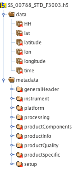
The Hierarchical Data Format (HDF) is the standard format of NASA’s Earth Observing System (EOS) mission. Its development by the HDF group is carried out through a subcontract under Raytheon Contract funded by NASA (The HDF Group, 2013).
The HDF5 datasets (.h5) provided by ASF are detected Seasat SAR images in ground range geometry. The layout of the Seasat HDF5 products is shown in Figure 1. It contains two groups: data and metadata.
The data group contains the SAR data as backscatter values in the HH layer. In order to provide basic geolocation information, two additional layers, latitude and longitude, are added. They contain geographic coordinates for every pixel in the image. The time variable completes the compliance to the Climate and Forecast (CF) metadata conventions (CF Conventions Committee, 2013).
The structure within the metadata group was modeled after the TerraSAR-X metadata (Astrium, 2013). The generalHeader section defines very basic metadata such as mission and data source. The instrument section summarizes radar parameters and settings. The satellite flight path with its orbital parameters is described in the platform section. The processing section provides vital information about Doppler as well as about processing parameters and flags. All product components are included in the productComponents section. The general product information is given in the productInfo section, while the SAR specific is stored in the productSpecific section
. Finally, the setup section provides details about data ordering and processing.
Users are advised that the Seasat HDF5 products may have substantial geolocation errors. The ASF Seasat HDF5 products have the file extension .h5.
11.2 XML Metadata
The same metadata structure that is stored in the HDF5 file is also saved as an XML file (.xml) and bundled with the ASF Seasat products. The XML (Figure 2) allows for simplified access and parsing of metadata information.
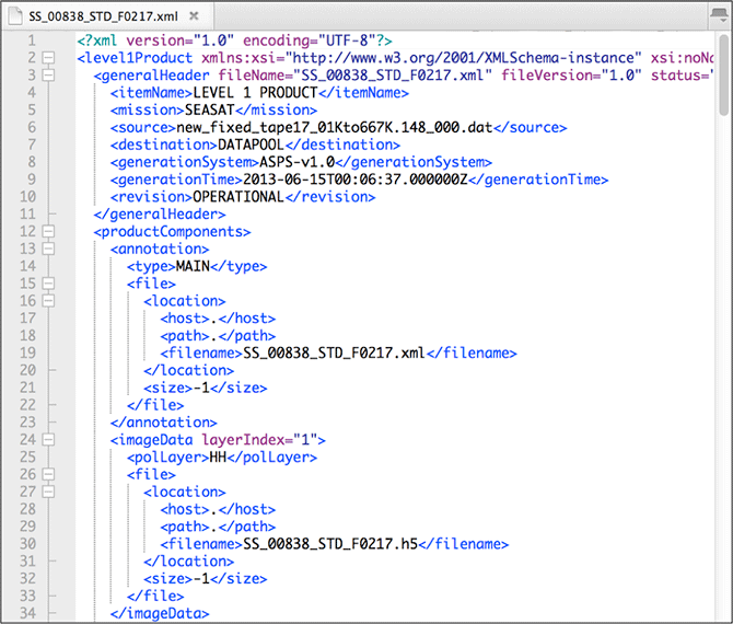
The development of XML metadata that is compliant to ISO 19115 and other related standards (NOAA EDM, 2013) is a work in progress. The SAR geometry is not comprehensively described with the current standard elements. In collaboration with Ted Habermann, now Director of Earth Science at The HDF Group, standards-compliant metadata for SAR data and best practices for future NASA missions are being developed. The current prototype structure is summarized in Figure 3. The ISO-compliant XML metadata files (.iso.xml), distributed as part of Seasat products, are considered experimental, and their structure is subject to change.
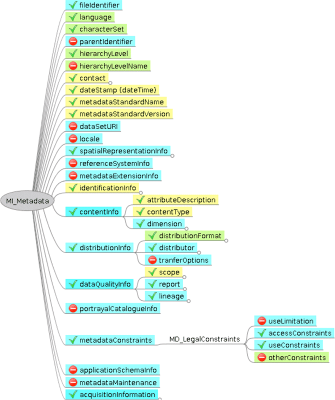
Figure 3: Prototype of an ISO 19115 compliant metadata structure for SAR data. Yellow backgrounds indicated mandatory elements, while green are conditional and blue optional.
11.3 GeoTIFF Products
GeoTIFF is a public domain metadata standard that allows georeferencing information to be embedded within a TIFF file. The GeoTIFF data products are geocoded to the Universal Transverse Mercator (UTM) map projection, using the zone that best represents the data’s geolocation. The original 12.5-m pixel size and the floating-point values of the ground range HDF5 products are kept in the GeoTIFF format. Because this product type does not require additional geographic information, it only contains a single layer of SAR data and is considerably smaller than the HDF5 product. Users are advised that the Seasat GeoTIFF products may have substantial geolocation errors. The ASF Seasat GeoTIFF products have the file extension .tif.
Written by Tom Logan, July 2013
Seasat – Processing and Tools
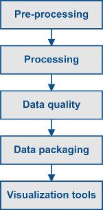
Cleaning and processing the original Seasat telemetry data presented challenges ranging from bit rot and data discontinuities to conflicting time records. Each step involved writing new software. When the telemetry data filtering was finished in the spring of 2013, 1,346 raw Seasat swaths were ready to be processed into synthetic aperture radar (SAR) image products. Engineers then turned their attention to the processing itself, and released beta products to commemorate the 35th anniversary of Seasat’s launch.
The following pages give an overview of the raw data preparation or pre-processing, image processing and product packaging. It is important to note that several data quality issues do exist in the resulting products — including imprecise geolocations and some image anomalies. There are some visualization tools that work with ASF’s Seasat HDF5 products.
Pre-processing
Seasat data were originally archived on 39-track raw data tapes. Years later, to ensure the preservation of the data, those tapes were duplicated in 1988 and again in 1999. During the second transcription, the raw telemetry data were transferred onto 29 more modern SONY SD1-1300L 19 mm tapes. Due to the transition of data through a number of different medias, special attention has been spent on cleaning the data during pre-processing.
In a first step, Seasat telemetry data were captured from the 19 mm tapes and byte-aligned using Vexcel’s SyncPrep tool. The raw telemetry data were then decoded into a format that a SAR processor could handle.
The decoded data was analyzed to get a first sense for the quality of the data. Pervasive bit errors, data drop outs, partial lines, discontinuities, and other irregularities were still present in the decoded data.
The many errors present in the Seasat raw data required multiple levels of cleaning and filtering before the actual SAR processing could be carried out. The time values needed special attention in this respect, since any further processing could not occur without this filtering step.
Median filtering was applied to metadata fields such as station code, least significant digit of year, day of year, clock drift, bits per sample, PRF rate code and delay to digitization. Linear regression was used to clean up the milliseconds of day metadata field. The linear regression needed to be refined in various ways. The measures to improve its robustness include restricting the time slope, removing bit errors from times, removing stair steps from times and removing time discontinuities.
Various time slope correction settings were used for the filtering and evaluated on a case-by-case basis. With another final level of filtering to fix bad start times, even more data was recovered. An example for cleaning a raw data set, as well as statistics on the amount of Seasat data recovered from tape and cleaned using these techniques, is given in the description of the Prep_Raw.sh cleaning script.
Several categories of bad data were identified during the analysis of the decoded and cleaned raw data: short files, constant time, random time, every other zero, time gap, time slope and wrong fix. Ultimately, this reduced the total amount of original Seasat data that could be processed to imagery by only a small fraction.
Processing
After the Seasat telemetry data was byte-aligned, decoded and cleaned, the raw data was ready to be processed into images. The Jet Propulsion Laboratory’s (JPL) repeat orbit interferometry (ROI) package was chosen to process the offset-video-format-encoded Seasat raw data. However, modifications were made to the processing system to improve the Seasat processing results.
ASF engineers evaluated the available sources for state vectors and chose the one that resulted in the best geolocation in the final products.
The Doppler value, a key parameter in describing the viewing geometry of the SAR sensor, is one of the most critical pieces of information for processing a data set into a focused image. Special attention is paid to the data quality analysis in order to detect ambiguities in the Doppler estimation. Ultimately, a visual inspection of each product determines if re-processing an image with a different Doppler value improves the focus of an image.
Range spectra filtering is applied to remove radio frequency interference. The delay to digitization — the time delay between transmitting and receiving a pulsed SAR signal — is adjusted on a regular basis. The required shifts are stored in a data window position file passed to ROI for processing.
The processing of the swath files into data products is carried out with the ASF Seasat Processing System (ASPS). ASPS uses the modified version of ROI to generate single look complex (SLC) images that are converted with ASF tools to the final detected ground range HDF5 products. The naming convention of the products follows
SS_ooooo_STD_Fffff,
where ooooo is the five digit orbit number of the Seasat satellite at the time of imaging and ffff is the four digit ESA frame number scheme, modified to create images 100 km x 100 km in size.
Data Quality
After pre-processing and processing of the data, there are remaining data quality issues to be aware of in the imagery. These anomalies result from sensor issues and processing limitations. All Seasat products can be searched and downloaded from ASF’s Vertex data portal.
Sensor anomalies are prevalent in Seasat data. One example is a calibration pulse that was introduced into the raw data in order to perform system testing. As a result, the majority of the Seasat imagery processed contains a very visible calibration pulse. Techniques for attempting to remove this calibration pulse from the data are currently under investigation. Another signal embedded into the raw data creates a set of short lines across the range direction. Attenuation, the gradual loss of image brightness across the image, appears in images from the first part of the Seasat mission, and it is possible that this effect may not be able to be removed from the data.
Image anomalies in the data are often introduced during acquisition or processing such as banding — a common result of missing data —, streaks in the along-track direction and streaks in the across-track direction. For Seasat data, the techniques for cleaning the raw data might have introduced additional artifacts. For example, only data with less than 4.5 percent partial lines actually focuses into valid imagery. Existing data gaps have been annotated in the metadata. When unfocused images are encountered during visual analysis, ASF re-processes the Seasat product with an adjusted Doppler value.
All available Seasat state vectors provide orbital information with an accuracy of several kilometers. Offsets were observed and have been mitigated by introducing an empirically determined slant shift of -1000 m. This shift resulted in geolocation errors in most cases on the order of 1 km or less. The introduced slant shift is going to be further investigated after more data sets are processed. Users are strongly advised to carefully evaluate the geolocation of individual data sets and should not expect that the geolocation accuracy is readily comparable to more recent SAR missions.
Finally, the data products can currently not be used for any quantitative analysis, since the ROI processor is not calibrated for Seasat data.
Data Packaging
The Seasat data product packages are distributed in two different formats: HDF5 and GeoTIFF. The files that are common to both packages, provided in the compressed .zip format, are the following:
- Browse image: SS_ooooo_STD_Fffff .jpg
- ISO XML metadata: SS_ooooo_STD_Fffff.iso.xml
- XML metadata: SS_ooooo_STD_Fffff.xml
- KML coverage file: SS_ooooo_STD_Fffff.kml
- Data quality report: SS_ooooo_STD_Fffff.qc_report
The Seasat HDF5 products contain two groups: data and metadata. The data group contains the SAR data as backscatter values and geographic coordinates. The structure within the metadata group was modeled after the TerraSAR-X metadata (Astrium, 2013). The ASF Seasat HDF5 products have the file extension .h5.
The GeoTIFF data products are geocoded to the Universal Transverse Mercator (UTM) map projection. The original 12.5 m pixel size and the floating-point values of the ground range HDF5 products are kept in the GeoTIFF format. Because this product type does not require additional geographic information, it only contains a single layer of SAR data and is, therefore, considerably smaller than the HDF5 product. The ASF Seasat GeoTIFF products have the file extension .tif. Users are advised that the Seasat products, whether in HDF5 or GeoTIFF format, may have substantial geolocation errors.
Visualization Tools
The Seasat HDF5 products are currently supported to varying degrees by a number of software packages that can be used to investigate and visualize the data.
The Geospatial Data Abstraction Library (GDAL) helps explore the general contents of the Seasat HDF5 data. The gdalinfo tool summarizes the data structure in the file. The gdal_translate tool can extract the SAR data out of the structure and store it into a more versatile GeoTIFF.
The commercial geographic information system ArcGIS recognizes the HDF5 structure and is able to extract the SAR data on the fly. The program does not calculate standard statistics for this data layer and is very slow in rendering the data this way. The handling of the data can be significantly improved by converting the HDF5 data layer HH into a GeoTIFF file using the gdal_translate tool.
The standard viewer of the MapReady tool suite offers the most comprehensive support for Seasat HDF5 data. It does not have any limitations for file size and provides the full functionality of asf_view, including sub-setting areas of particular interest.
HDFView, provided by the HDF group, has two different ways to look at the data. For any quantitative analysis, the selected data layer needs to be opened as a spreadsheet. For a more visual analysis, HDFView provides the image view. The program has no options for stretching the data in a statistical fashion. However, the user can manually change the brightness and contrast.
Panoply, developed by NASA’s Goddard Institute for Space Studies, is primarily used for global data sets of lower resolution, and visualizing Seasat HDF5 with it is difficult. The rendering at 12.5 m pixel size requires working with a subset of the Seasat HDF5 product.
The Interactive Data Language (IDL) provides a more programmatic means to visualize the Seasat HDF5 data. The IDL H5 browser has very limited functionality in terms of changing visual value ranges and stretching the imagery for visualization purposes but does provide users the ability to view the HDF5 products.
Data Product Formats
The Seasat HDF5 products are currently supported to varying degrees by a number of software packages that can be used to investigate and visualize the data.
The Geospatial Data Abstraction Library (GDAL) helps explore the general contents of the Seasat HDF5 data. The gdalinfo tool summarizes the data structure in the file. The gdal_translate tool can extract the SAR data out of the structure and store it into a more versatile GeoTIFF.
The commercial geographic information system ArcGIS recognizes the HDF5 structure and is able to extract the SAR data on the fly. The program does not calculate standard statistics for this data layer and is very slow in rendering the data this way. The handling of the data can be significantly improved by converting the HDF5 data layer HH into a GeoTIFF file using the gdal_translate tool.
The standard viewer of the MapReady tool suite offers the most comprehensive support for Seasat HDF5 data. It does not have any limitations for file size and provides the full functionality of asf_view, including sub-setting areas of particular interest.
HDFView, provided by the HDF group, has two different ways to look at the data. For any quantitative analysis, the selected data layer needs to be opened as a spreadsheet. For a more visual analysis, HDFView provides the image view. The program has no options for stretching the data in a statistical fashion. However, the user can manually change the brightness and contrast.
Panoply, developed by NASA’s Goddard Institute for Space Studies, is primarily used for global data sets of lower resolution, and visualizing Seasat HDF5 with it is difficult. The rendering at 12.5 m pixel size requires working with a subset of the Seasat HDF5 product.
The Interactive Data Language (IDL) provides a more programmatic means to visualize the Seasat HDF5 data. The IDL H5 browser has very limited functionality in terms of changing visual value ranges and stretching the imagery for visualization purposes but does provide users the ability to view the HDF5 products.
Seasat Images Then and Now
| Images Then and Now |
|---|
| The Washington-Oregon coast |
| These images, acquired nine days apart, both show the influence on wave patterns of a subsurface sediment spit near the mouth of the Columbia River between Oregon and Washington. The river is one of the largest in the world without a delta. The optically processed image to the left was acquired from Fu, L.-L., and B. Holt, “Seasat Views Ocean and Sea Ice with Synthetic-Aperture Radar,” Publication 81-120, Jet Propulsion Laboratory, Pasadena, Calif., 1982. |
| Washington-Oregon coast: optically processed in 1982 |
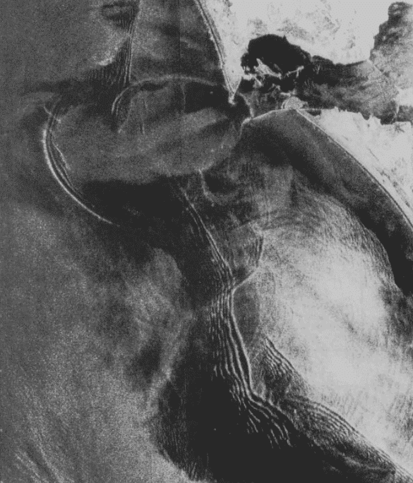 |
| Acquisition date: August 19, 1978, Processing organization: JPL, NASA/JPL |
| Washington-Oregon coast: digitally processed in 2013 |
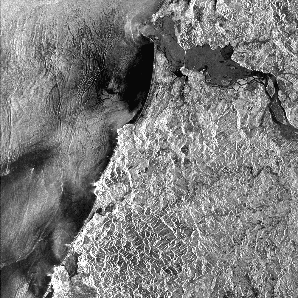 |
| Acquisition date: August 10, 1978, Processing organization: JPL, NASA/JPL |
| The Kuskokwim Delta |
| Two Seasat SAR images, digitally processed 26 years apart, highlight advances in digital processing techniques and data storage technology. These advances allow more Seasat data to be processed and readily available for quantitative analysis to users around the world. The white line in the image to the right is from a calibration pulse. |
| Kuskokwim Delta: digitally processed in 1987 |
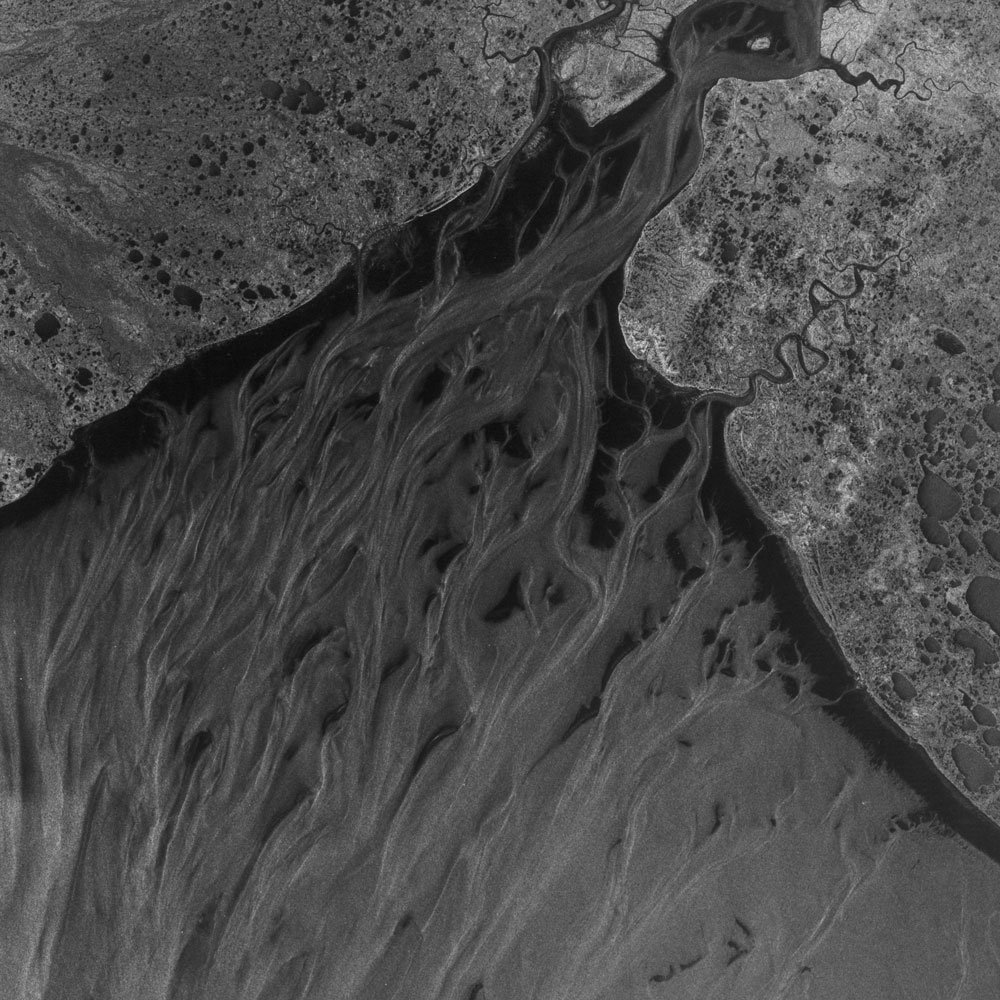 |
| Acquisition date: August 19, 1978, Processing organization: JPL, NASA/JPL |
| Kuskokwim Delta: digitally processed in 2013 |
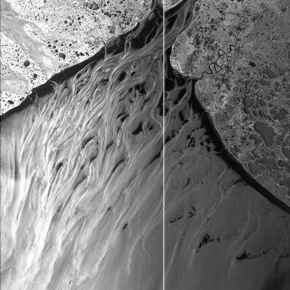 |
| Acquisition date: July 13, 1978, Processing organization: JPL, NASA/JPL |