
Alaska is losing about 50 cubic km of ice per year, but much of the new-water sea-level rise expected over the next 100 years may come from changes in mountain glacier calving and ice flow, which are completely unconstrained and unincorporated into mass loss projections.
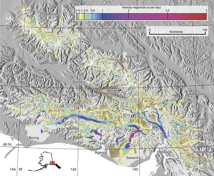
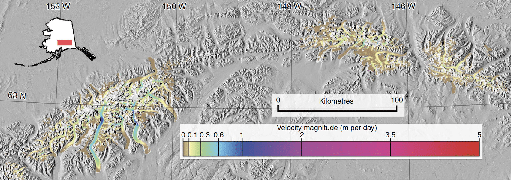
Over half of the downstream ice flux from more than 20,000 glaciers throughout Alaska comes from fewer than 12 coastal glaciers. The flow dynamics on these rapid-flow systems will operate differently than from those of other glaciers, because they are able to maintain higher flow speeds without losing mass. Understanding the dynamics of these glaciers is critical for future efforts to estimate flow-speed-related mass loss in Alaska.

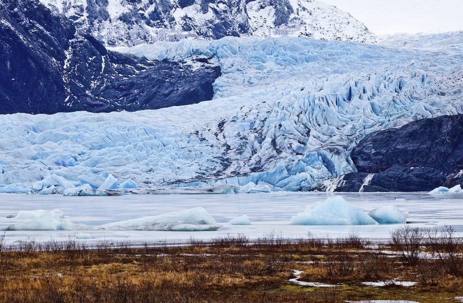
Icebergs float from the calving Mendenhall glacier, which originates in Alaska’s Coast Range. The glacier velocity dataset reveals that about 40 percent (approximately 20 cubic km) of ice lost annually in Alaska is due to calving alone, mostly from a few coastal glaciers. © UAF Improving projections of future sea level rise will require a thorough understanding of how climate change will affect glacier flow speeds. Flow speeds of ocean-calving glaciers originating from ice sheets have been closely monitored for many years, leading to better understanding of ocean-ice sheet interactions. But flow velocities of mountain glaciers have not been as widely monitored as ice sheets, and current projections of mountain-glacier mass loss are limited to extrapolating melt and snowfall observations on only a few glaciers to large regions.