
First, the header file (.hdr file) is read and decoded. Some of the fields in the header are supposed to have constant values throughout each datatake, and these field values are cleaned before those of the time-dependent fields. Examples of these constant fields include bandwidth, beam spoiling, beam width, command type, data format, datatake number, operational mode, orbit number, polarization, pulse repetition frequency (PRF), and pulse width. The values of these fields were recorded for each pulse return, and many of the recorded values are incorrect due to bit error. By assuming that the bit error has a random distribution, the values in each constant field can usually be cleaned by setting all of them equal to their statistical mode (the value that occurred most often in each field). The resulting values for data channel number (DDHA_ID), datatake number, and orbit number are verified by comparing them to the corresponding information in the input filenames.
Next, the pulse offset file (.pof file) is used to determine the number of lines within the datatake and to extract the pulse repetition frequency (PRF). The frame counts are compared from the header file and from the pulse offset file and used to identify the locations where lines are missing. The size of each field is expanded and padded for missing lines.
We then turn our attention to the 1-sec durations between the starts of each second. The MET (Mission Elapsed Time) is used to preliminarily identify the beginning and end of each 1-sec of data. For 1-sec durations in which the PRF does not match the number of signal returns (after accounting for missing lines), attempts are made to fix the delineation between seconds without altering the 1-sec durations that did contain a match. Next, using the updated delineation, we identify the largest set of consecutive 1-sec durations that each contain the proper number of signal returns equal to the PRF at that time. For each of the 1-sec segments in the consecutive set, the one second time tick (OSTT) is updated with the appropriate square wave and the MET is updated with a whole number indicating time in truncated seconds. Using these updated time fields, we then clean the fields that can change value throughout a datatake but should remain constant between the one second ticks. These fields include data window position (DWP), data window position time, (DWP Time), antenna mechanical tilt angle, azimuth angle, range angle, and gain. All of these fields except for DWP Time are updated with their statistical mode over the 1-sec durations. The DWP Time is cleaned using the updated DWP values and the following formula: DWP Time = 448/STALO*DWP in which STALO = 89,994,240. Note: to avoid confusion and to simplify the coding process, the 8-sample lead often observed in header fields such as DWP, DWP Time, and PRF is identified, accounted for, and removed at this stage in the cleaning process. Finally, the telemetry data are cleaned in a piecewise manner first by using standard deviation to identify significant outliers, then by using linear regression and median filtering to identify minor outliers, and lastly by sampling a cubic curve fit to the non-outliers.
After the header fields are cleaned, we identify the beginning and end of the datatake acquisition. This is accomplished by recognizing PRF hops within the aforementioned set of consecutive 1-sec durations that each contain the correct number of lines equal to the PRF value for that duration. In principle, there should be two PRF hops (each 2 seconds long and containing two different PRF values: PRF-A and PRF-B) that denote the beginning and end of the datatake acquisition. If there are no PRF hops within the set, then the entire set is processed to generate an image. If there is only one PRF hop in the set, then the longer of the two subsets before and after the hop is used. If there are three or more PRF hops, then the longest subset between hops is used. Note that there exists a single-bit header field named “data take enabled” that should identify the beginning and end of a datatake, however its values have been found to be unreliable and it is therefore not used in the cleaning process. Missing and partial lines are identified and filled with random noise. The seeding of the random noise ensures that this step is reproducible. Finally, the orbit information is retrieved.
SIR-C Table 1 – Header Contents
 |
| Table 1: SIR-C header contents (64 bytes in total). Each small cell (one row x one column) represents one byte in size. All parameters with gray highlighted background are cleaned as part of the preprocessing step. |
The data are converted from their original demultiplexed header/signal data format (.dmx file) by channel into a chronological order for each polarization and band. Each image is then divided into smaller sub-images of 21,000 lines for the SAR processing step. The sub-images overlap by 1,000 lines. Finally, the state vector information is propagated to each line.
Pitch and yaw calculation
In preparation for the actual SAR processing, pitch and yaw values throughout a datatake are estimated by stepping a 10,000-line window in steps of 2,000 lines through each band and polarization. For each line in a window, pitch and yaw angles are estimated from the difference between the estimated Doppler centroid and the calculated Doppler centroid. Then, a single least-mean-square estimate for each window for both pitch and yaw is made using only those of the 10,000 pitch and yaw estimates within the window that do not have clutter-to-noise ratios that are too large or too small. Using the least-mean-square estimates at each window center 2nd degree polynomials (quadratic curves) are fitted to the estimates for both pitch and yaw. Final pitch and yaw values are determined at the center of each 20,000-line image by evaluating both polynomials at each image center.
SIR-C SAR Processing
 | The processing for the SIR-C data is performed using a standard range Doppler processor concept. The main processing steps are the following: (1) the data are initially shifted to baseband to ensure that the mean value of the data is around zero using a Hilbert transform; (2) the data are first compressed in range by multiplying data with the complex conjugate of a weighted reference function in the frequency domain. The weighted reference function is calculated by multiplying the range reference function by a cosine square filter with a 0.45 pedestal in the time domain (described in more detail in the next section); (3) the range cell migration corrects the range dependent velocity in frequency domain, straightening out the range lines. The Doppler centroid is determined along the entire data take, in samples of 21,000 pulses with an overlap of 1,000 pulses. The data are then shifted to zero Doppler correcting for Doppler variation in range; Finally, (4) the data are compressed in azimuth direction. The data are multiplied with the complex conjugate of the weighted azimuth reference function in the frequency domain. As in the range direction, the weighted reference function is calculated in the same way in time domain. |
|---|
The JPL documentation suggested the use of a cosine square window with a 0.45 pedestal in both azimuth and range direction. After some testing, the team decided to follow this suggestion both for the azimuth and range reference function. The range profiles of the point target below show the expected behavior. The windowing suppresses the sidelobes at the expense of some resolution (Figure 1). A more detailed analysis of impulse response functions is shown in the following section, where point targets are analyzed to assess the focusing quality achieved by the processor.
SIR-C Figure 1 – Range Profile
 |
| Figure 1: The plots show range profile without windowing (left) and with a cosine square window with a 0.45 pedestal (right). The windowing suppresses sidelobes while losing resolution. |
SIR-C Table 2 – Pont Target Analysis
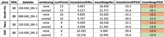 |
| Table 2: Point target analysis results of three study sites. The results of two different windowing options are compared. For each option resolution and PSLR are determined in azimuth and range direction. |
The point target analysis of data from three different areas shows that the mean range resolution decreased when applying the window (Table 2). The mean range peak-to-sidelobe ratio (PSLR) is below the required level of -17 dB (Freeman et al., 1995).
While the PSLR meets the requirements in the Freeman paper, the resolution does not quite match the goals (9 m for 20 MHz results and 18 m for 10 MHz in range direction).
The purpose of the antenna elevation pattern correction is to remove the impact of the antenna characteristics from the acquired SAR image data. A popular approach for antenna pattern estimation and verification is to use acquisitions over a large homogeneous rain forest area in the Amazon basin and estimating deviations from a flat SAR image brightness response in range direction.
The ASF team implemented a two-pronged approach based on in-orbit antenna pattern estimates on one hand and beam nulling on the other. Beam nulling is a calibration method employed by SIR-C, which involved inverting the receive phase of half of the antenna array in elevation by 180 degrees. Thus, the effective beam received has a notch or null at the boresight.
ASF’s final implementation of the antenna pattern correction algorithm was tested on a total of 12 real SIR-C datatakes, which equates to about one terabyte of raw data. The test results were found to be consistent with original JPL technical reports and show that the antenna model approach was successfully applied (Figure 2). In-orbit measurements of the residual relative radiometric cross-swath errors after antenna pattern correction were better than ± 1 dB, with best case scenarios as low as ± 0.11 dB over the Amazon rainforest.
SIR-C Figure 2 – Antenna Elevation Pattern Correction
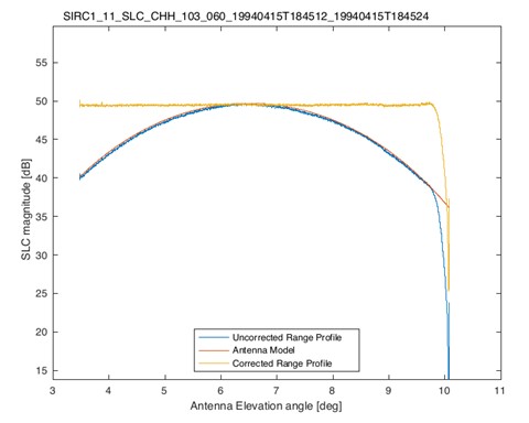 |
| Figure 2: Antenna elevation pattern correction over an Amazon rainforest image. The uncorrected range profile is shown in blue. The antenna model fitted to the profile (red) is used to calculate the corrected range profile (yellow). |
Calibration
For calibrating the processor, and converting the measured digital number data into calibrated radar cross section information, a calibration factor needed to be determined. Our current approach for image calibration is to calibrate the individual polarimetric bands of the SAR data takes independently. As the calibration factor depends on beam mode and polarization, separate data takes acquired over the Amazon rainforest were selected for each SIR-C beam mode (Figure 3). The scaling factors are determined separately for each polarization of a beam mode.
These are the three images that have been used for calibration of modes 11, 16 and 20:
SIRC1_11_SLC_103_060_001_19940415T184512_19940415T184524
SIRC1_16_SLC_007_030_003_19940409T203803_19940409T203815
SIRC2_20_SLC_119_040_032_19941007T183706_19941007T183721
SIR-C Figure 3 – Calibrated Pixel Values
 |
| Figure 3: Calibrated pixel values along an averaged range profile. Once the calibration factor is applied, the mean value of the scene needs to be -6.5 dB while having a narrow range profile. |
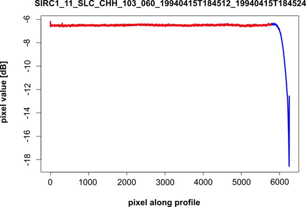
The processing leads to a power loss in the far range, caused by the fact that there is not enough data left to be multiplied by the range reference function. To remove these invalid data, all images are cut in far range by the number of samples equivalent to the length of the respective reference function (Figure 4).
SIR-C Figure 4 – Corrected Range Profile.
|
| Figure 4: Antenna elevation pattern corrected range profile. The data are acquired with the original width of 6254 samples. Based on pulse duration and range sampling rate, the length of the range reference function is 380 samples (blue) and the resulting image width is 5874 samples (red). |