
There are two sample Geocoded Covariance (GCOV) products available, one for each of the acquisitions used in other sample products that require imagery pairs:
NISAR_L2_PR_GCOV_001_030_A_019_2000_SHNA_A_20081012T060910_20081012T060926_D00402_N_F_J_001.h5
NISAR_L2_PR_GCOV_002_030_A_019_2000_SHNA_A_20081127T060959_20081127T061015_D00402_N_F_J_001.h5
The covariance variables are essentially equivalent to Normalized Radar Backscatter (NRB) or Radiometrically Terrain Corrected (RTC) products. They include additional information that make them suitable for additional analysis workflows beyond what a standard RTC product can be used for, but can also simply be used in place of an RTC.
The illustrations displayed in this section use the acquisition from October 12, 2008. Note that the data used to create these sample products are from JAXA’s PALSAR sensor, which also operates in the L band, but the product has a smaller footprint than the NISAR acquisitions.
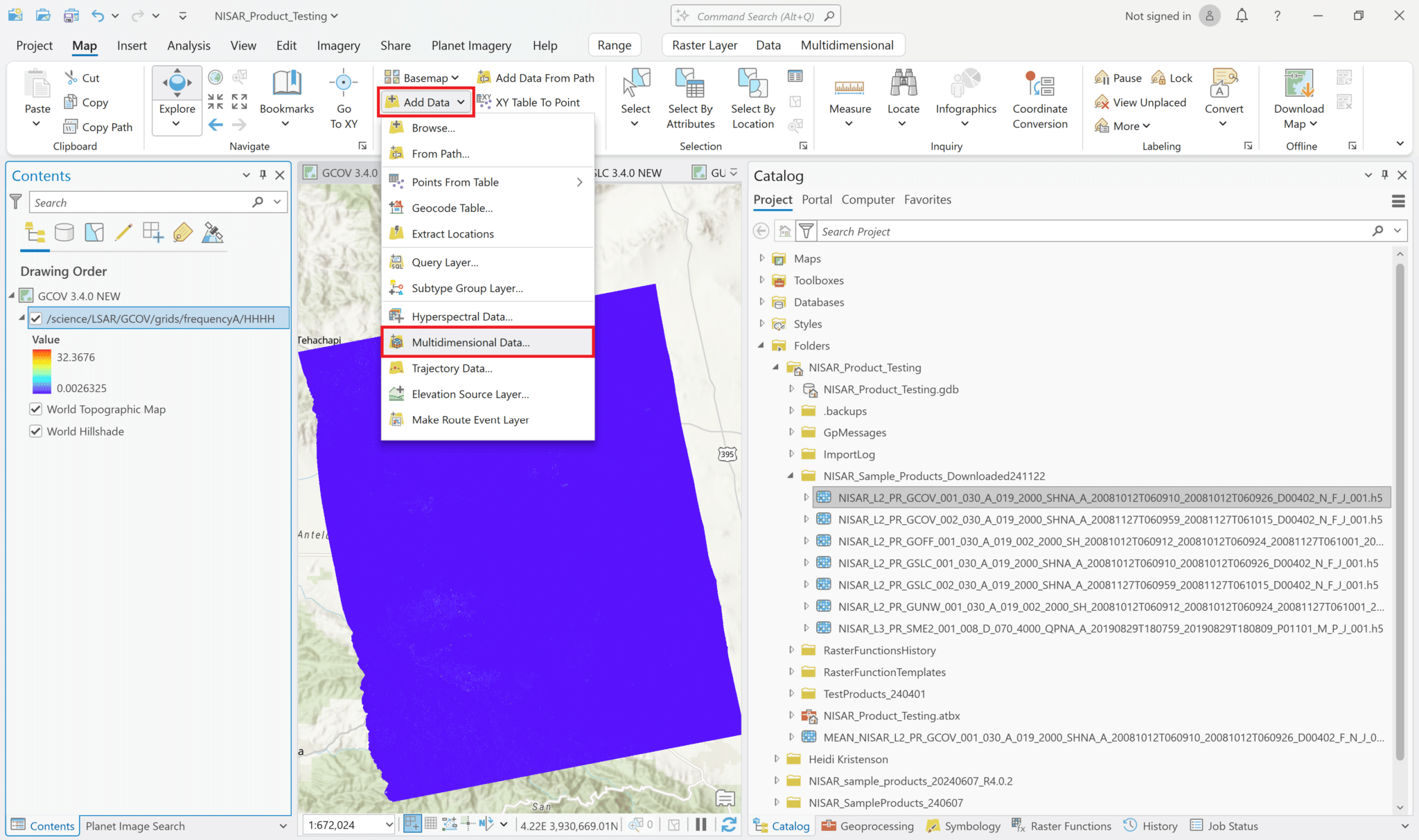
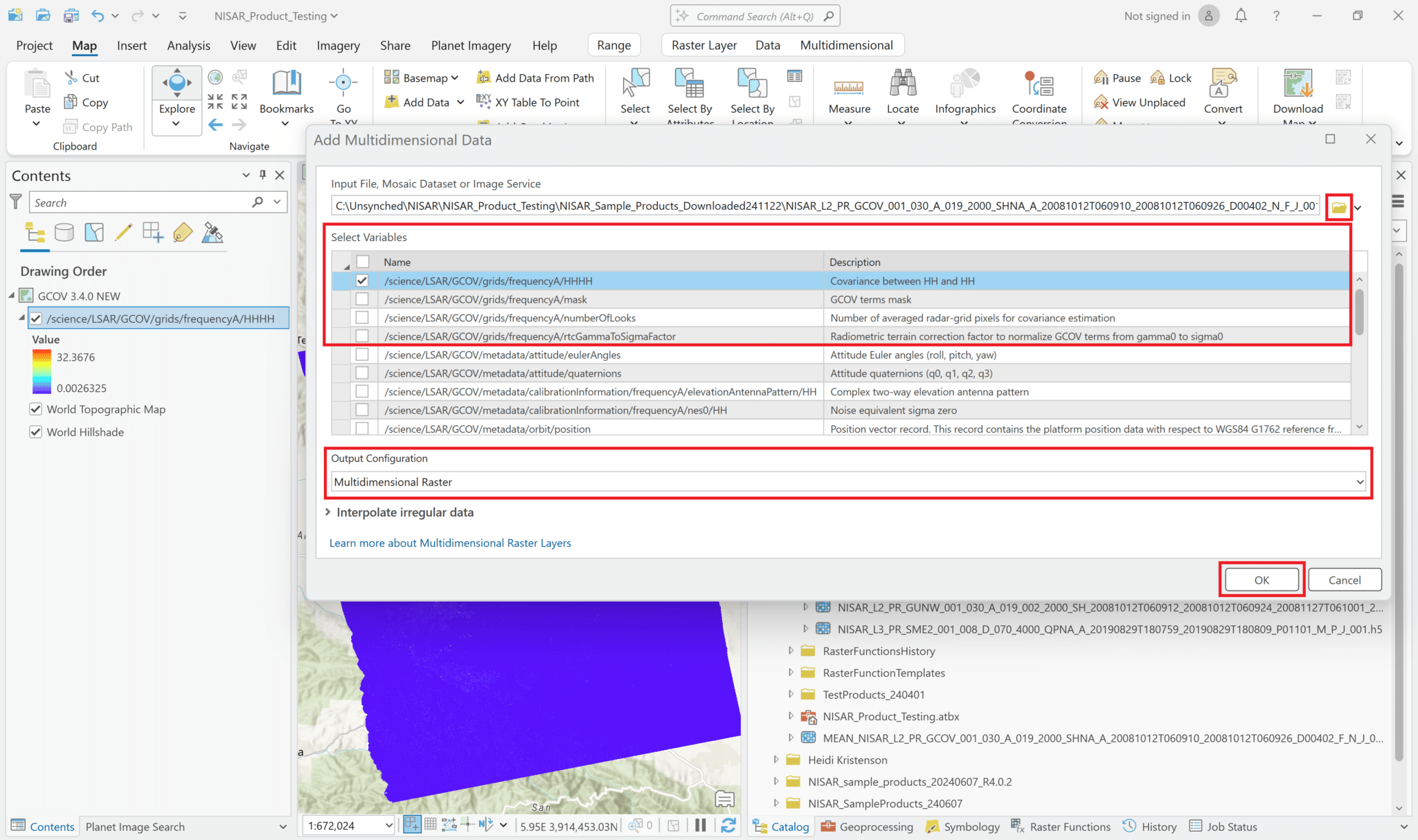
Add GCOV Data
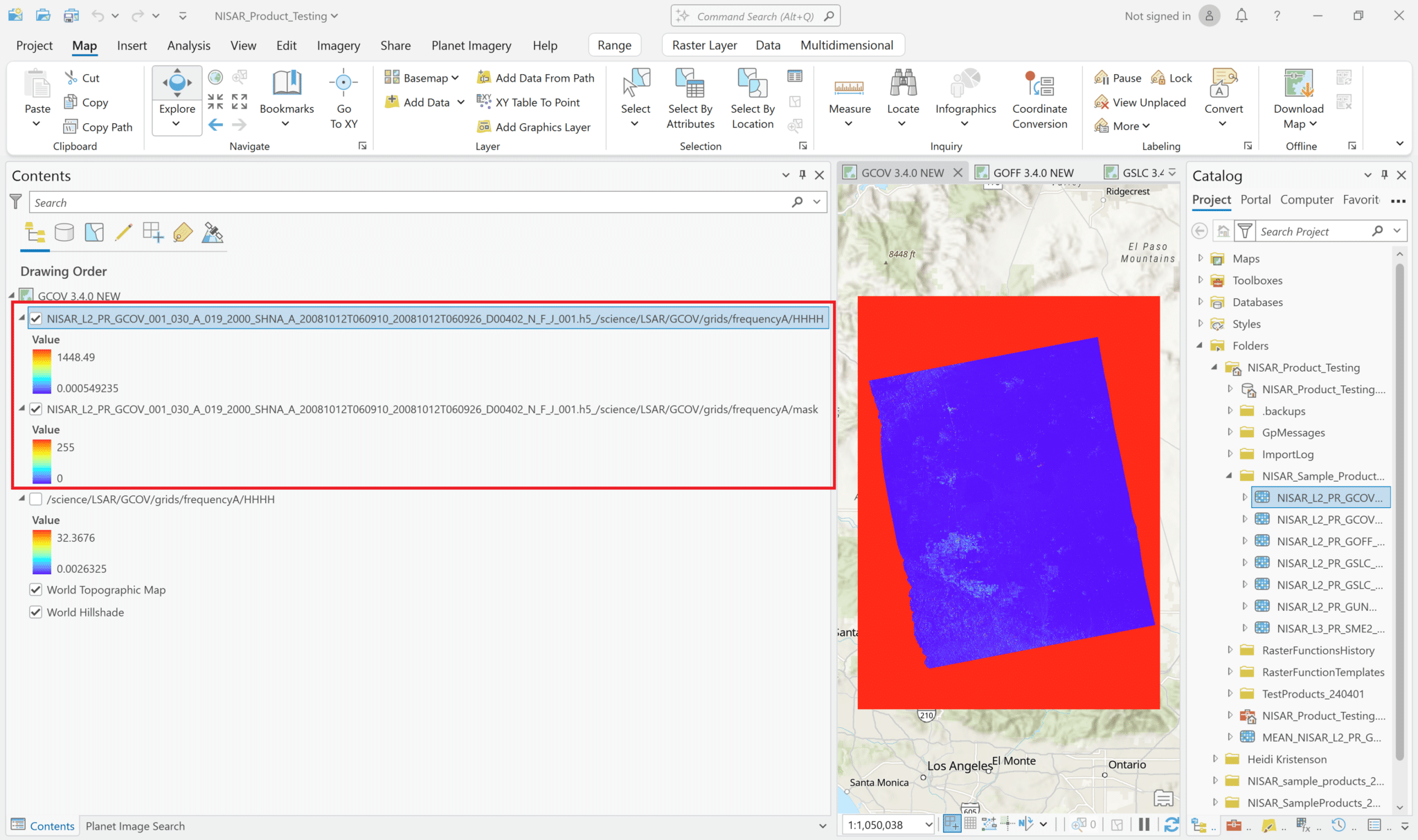
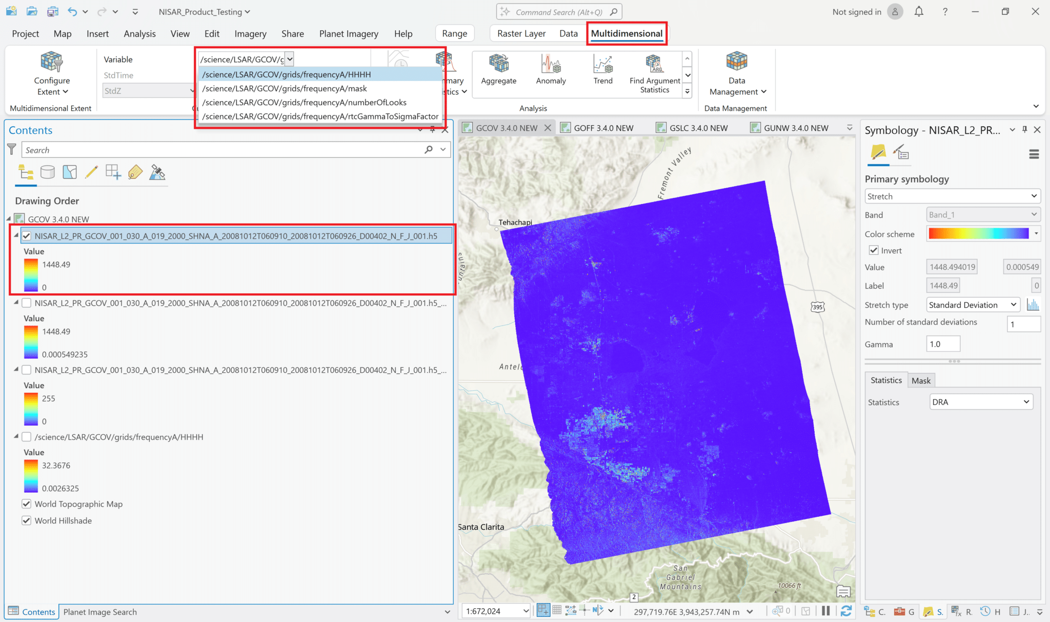
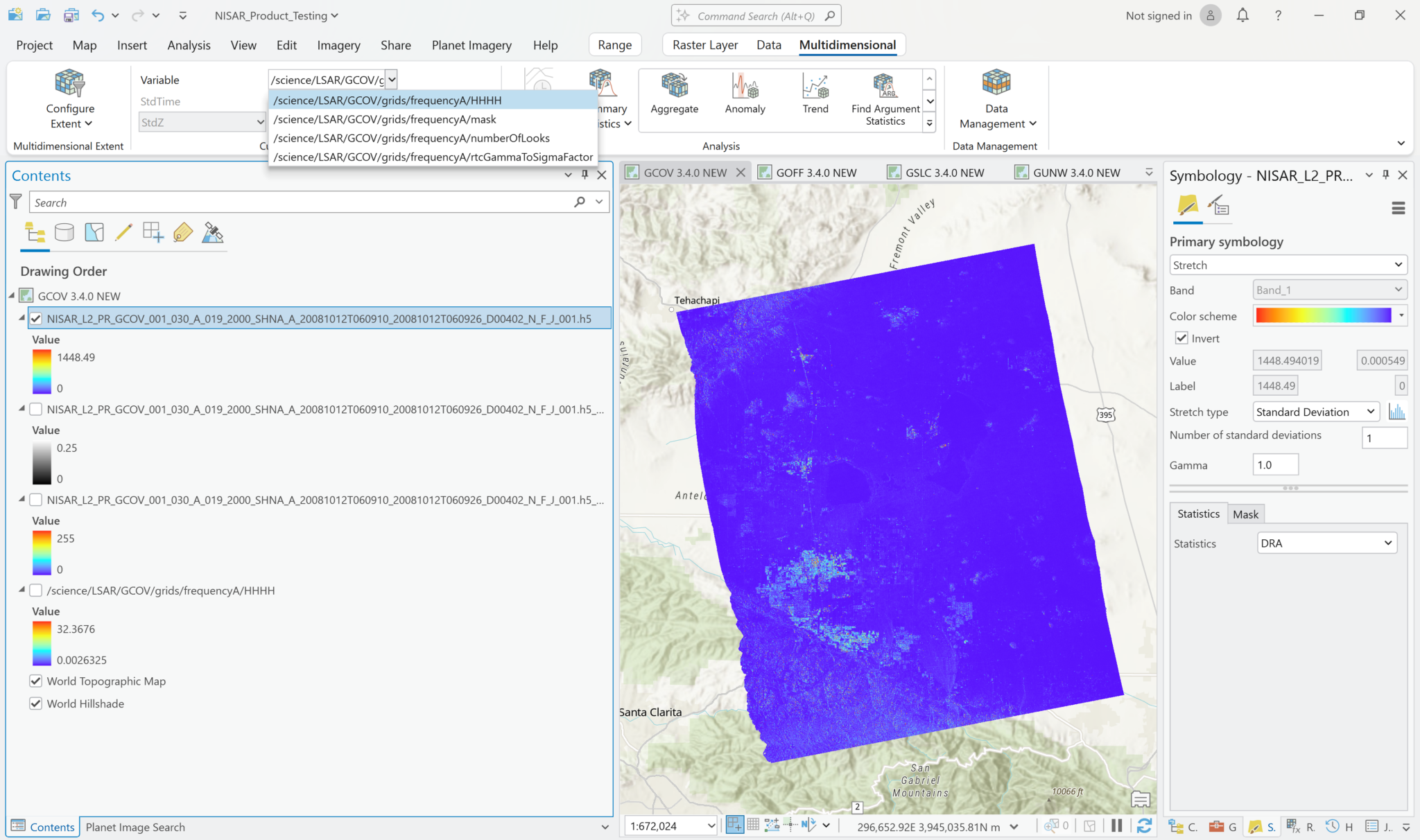
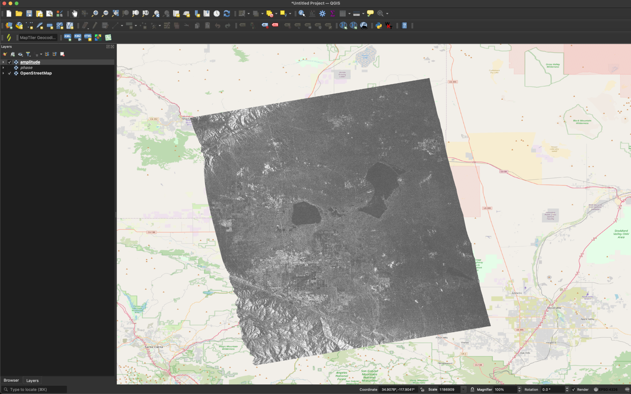
You can use any of the standard methods to add GCOV products to your ArcGIS Pro map. If you drag and drop, the HH-HH covariance variable will be displayed by default.
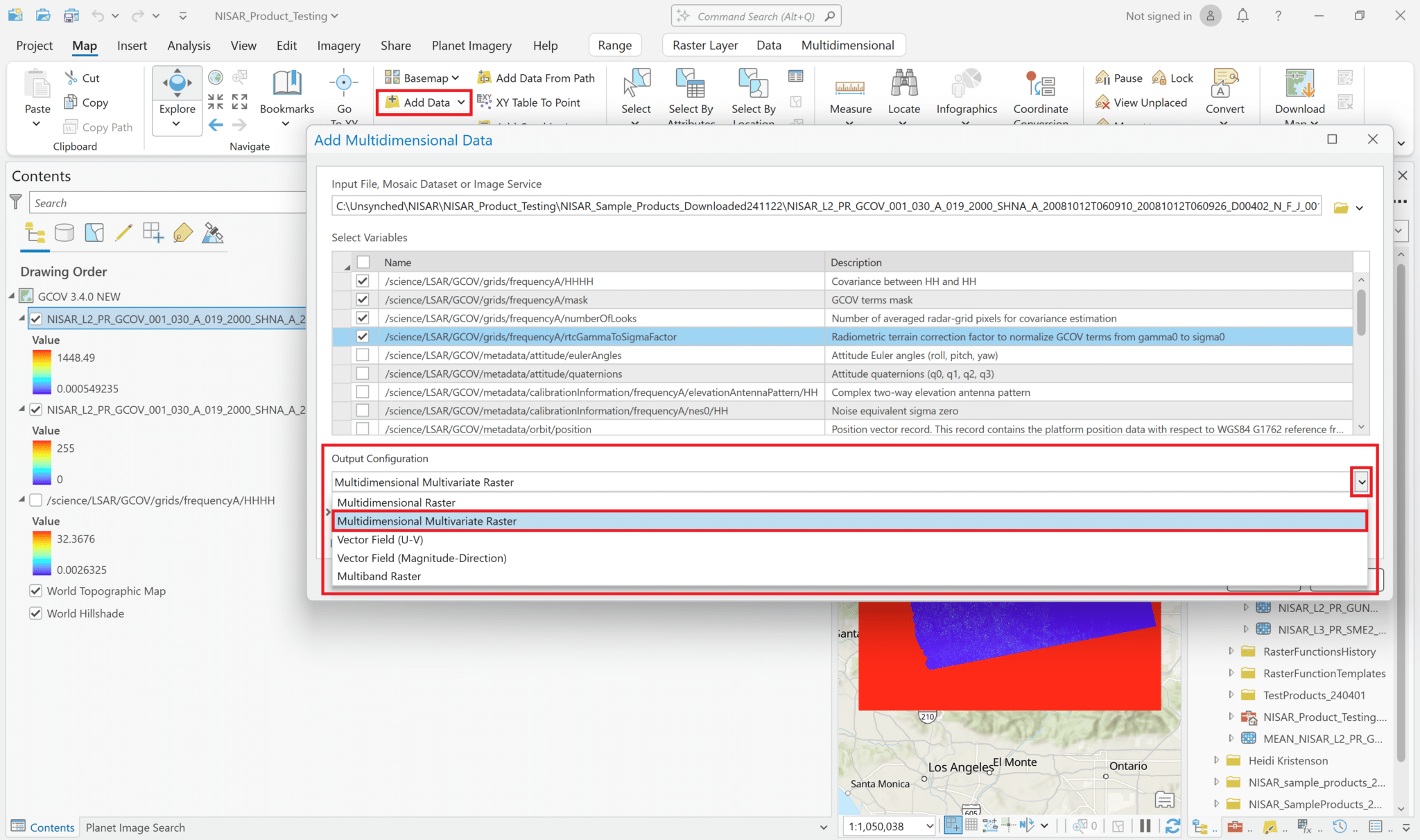
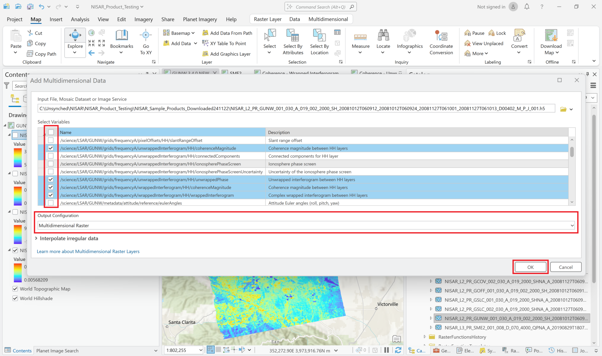
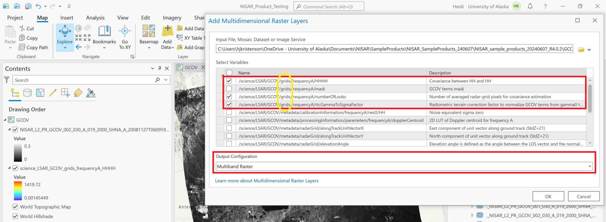
When using the Add Multidimensional Data dialog, any of the variables in the grids path of the file can be added to the map, but most users will be interested in viewing the Covariance layers.
Note that the sample data only includes one polarization (HH). Most NISAR data will include at least two polarizations (over land, most acquisitions will include at least HH and HV), and each will be included as a separate variable in the h5 file.
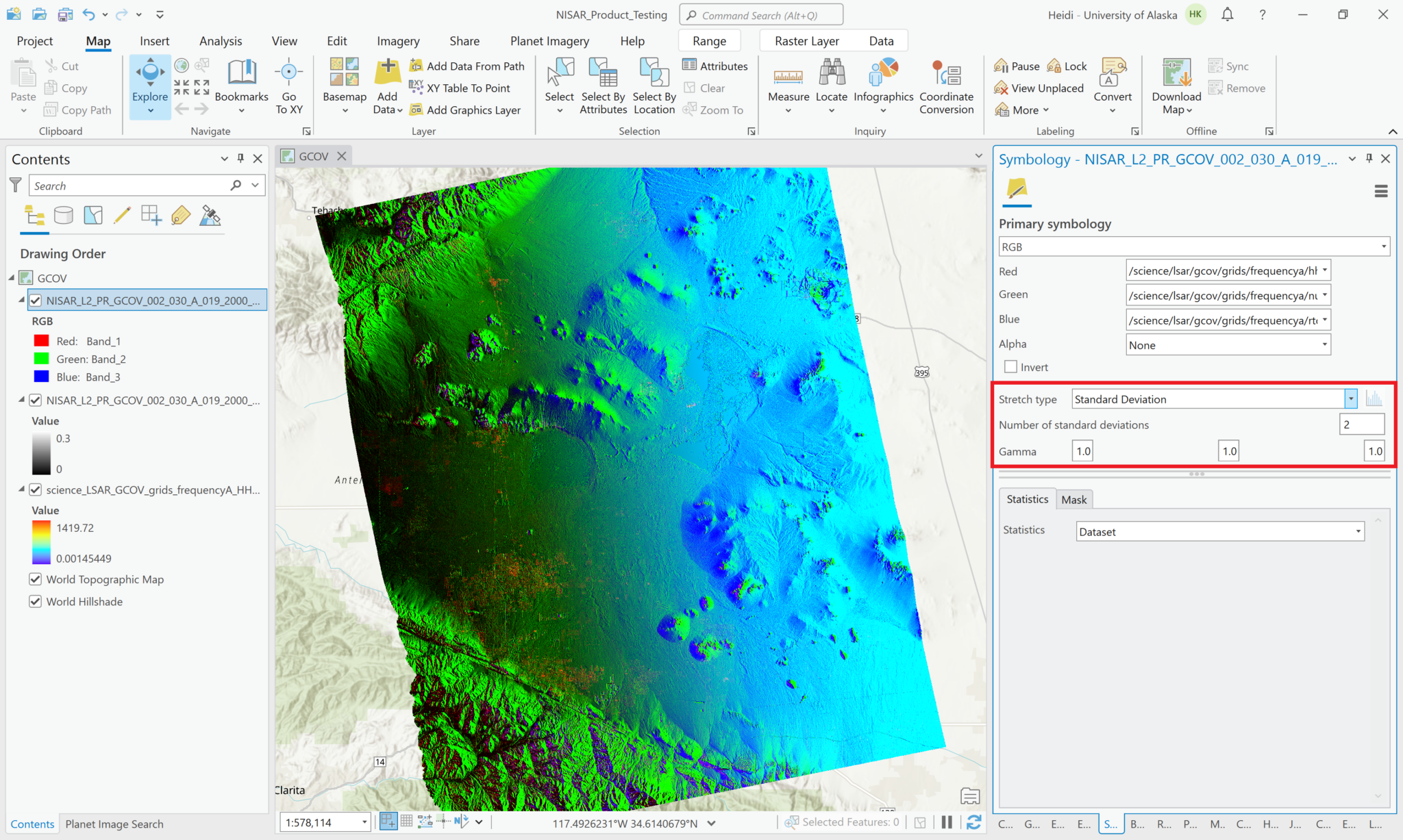
Visualize GCOV Products
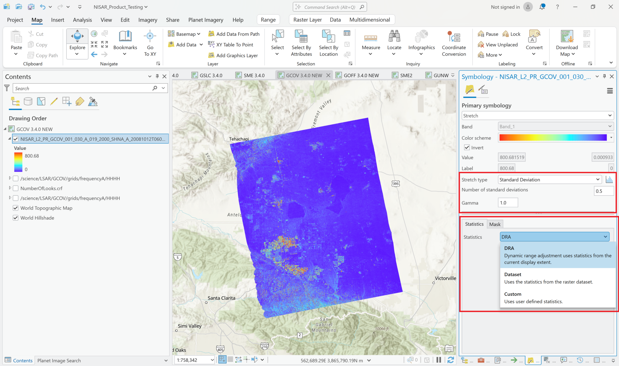
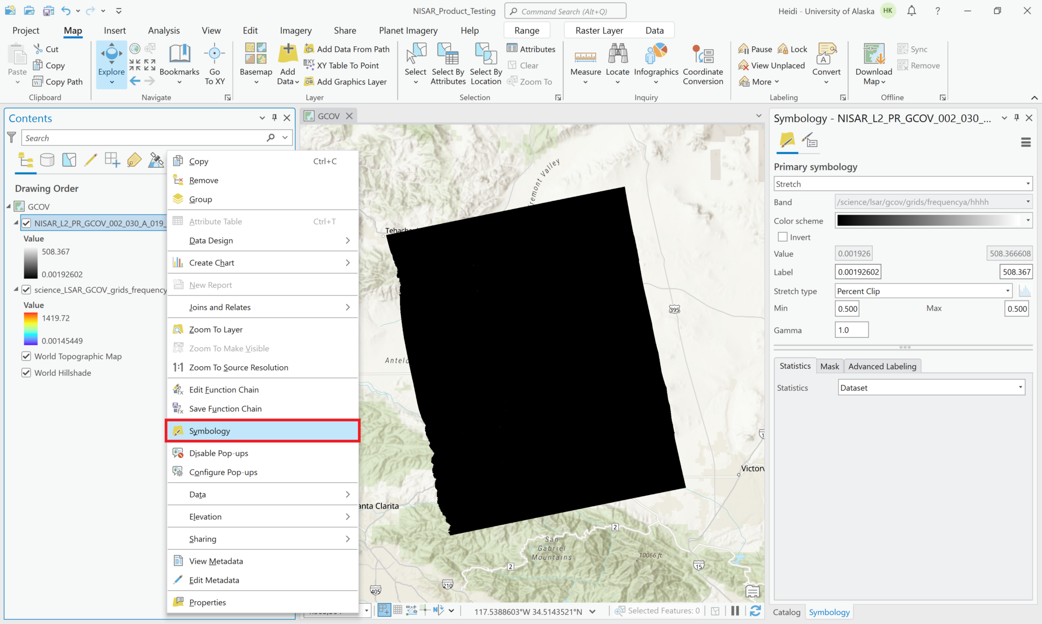
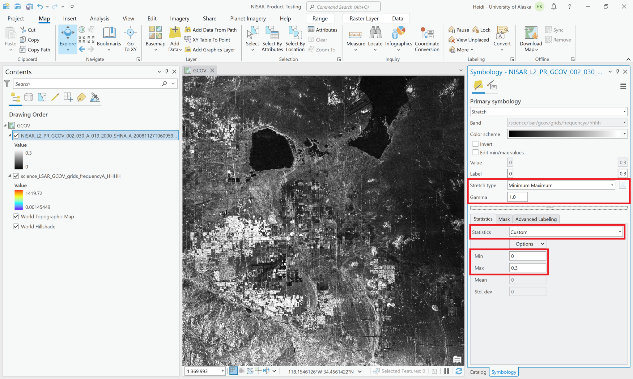
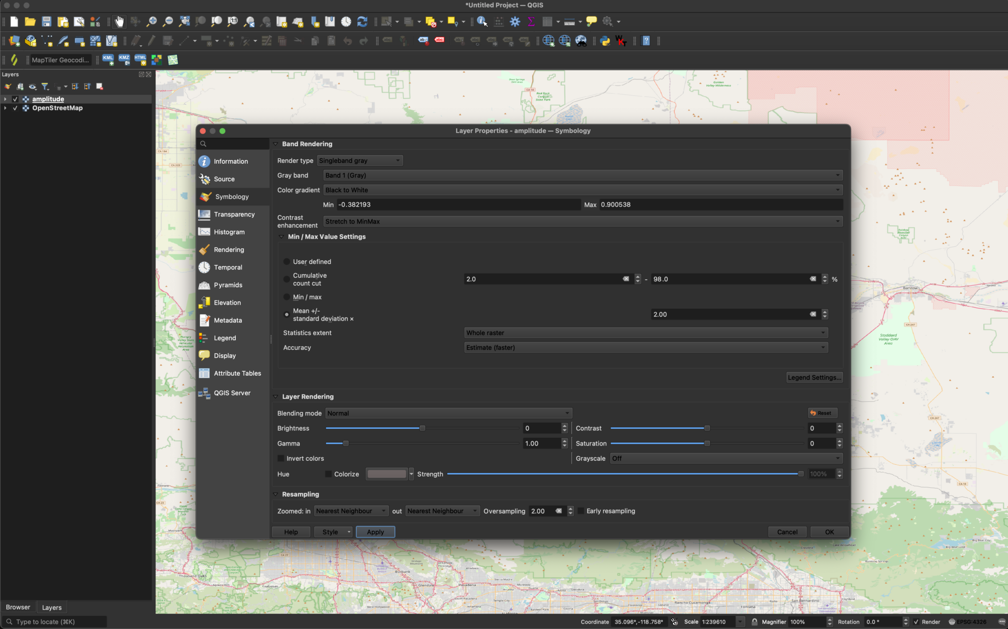
You can adjust the symbology of the NISAR sample data layers just like you would any other raster layer. Right-click the layer in the Contents pane, and select Symbology. Adjust the stretch as desired. If you are accustomed to looking at RTC products in grayscale, set the color scheme to Black to White, and make sure that you uncheck the box to invert the color direction.
Common approaches for backscatter stretch settings are to use a Minimum-Maximum stretch with fixed values applied (i.e. 0 to 0.25), or to use a Standard Deviation stretch, choosing an n value that works well for your particular image.
If you’ve used the Multivariate approach to add multiple variables with different value ranges to a single Multivariate layer, recall that the same symbology will be automatically applied to each of the layers when you select a different variable. In this case, you may want to use a Standard Deviation stretch rather than a Min-Max, as it will accommodate a wider range of values. Consider also using the DRA (Dynamic Range Adjustment) setting for statistics rather than the dataset statistics.
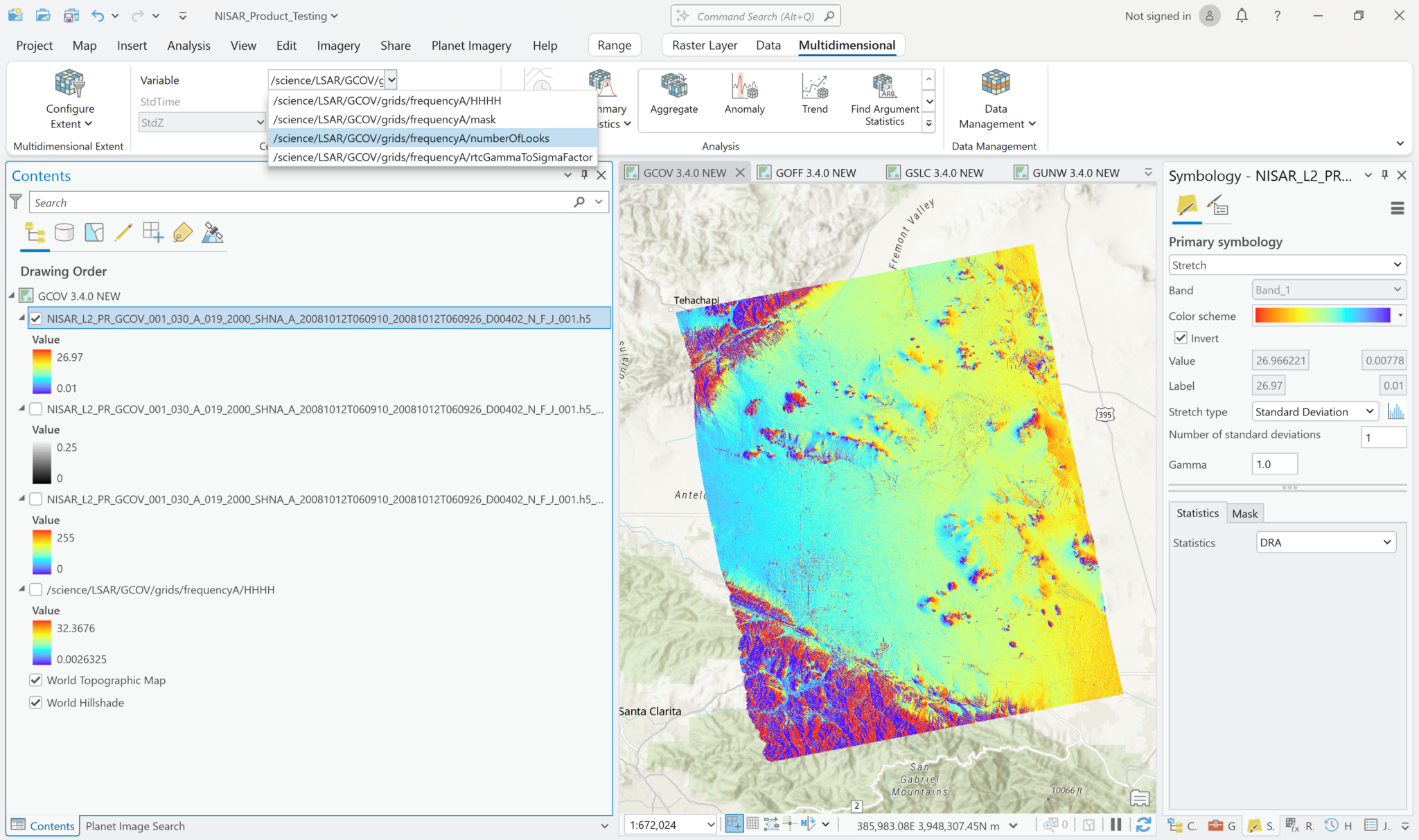
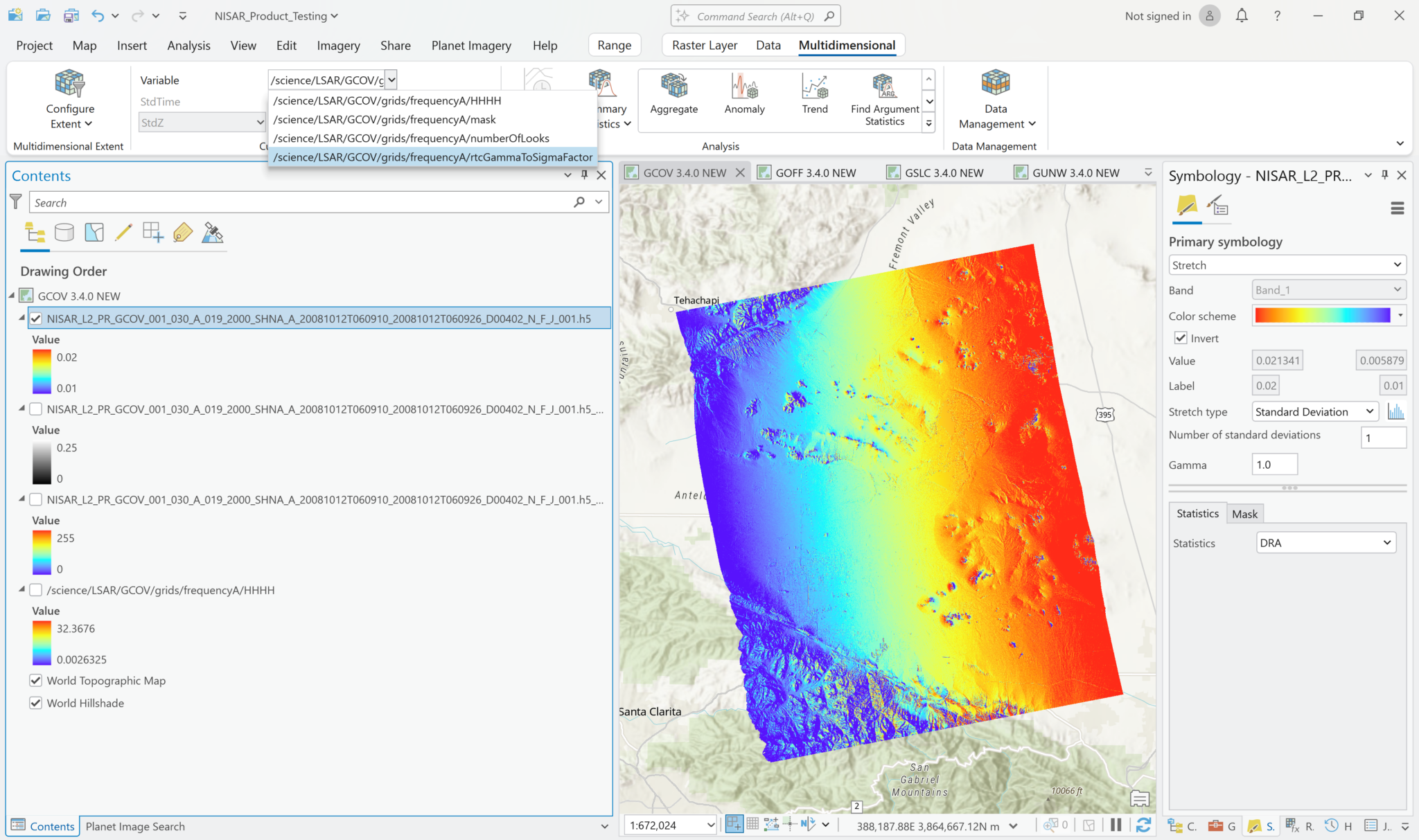
The following series of screen shots displays all the different GCOV sample data grid variables using the same stretch setting.
Multiband Raster Symbology
While this is not a particularly compelling approach for the current sample GCOV data, which only includes one polarization for covariance, it is possible to add multiple covariance variables from a single HDF5 file to your project as a Multiband raster. Once data files are available that include multiple polarizations, you will be able to use this feature to generate RGB images by assigning different polarizations to different bands (i.e. set the Green band to use the HV variable and the Red and Blue bands to use the HH variable).
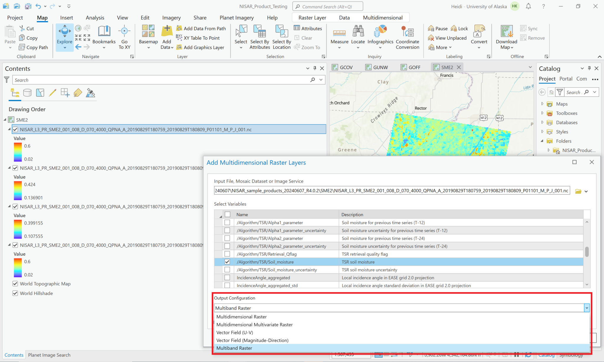
To use this functionality, set the Output Configuration to Multiband Raster when selecting the variables to add to the map. This adds a single layer to the map, with the individual variables available as bands in the Symbology interface.
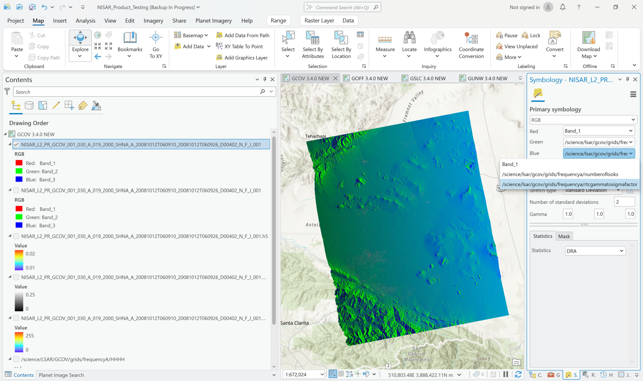
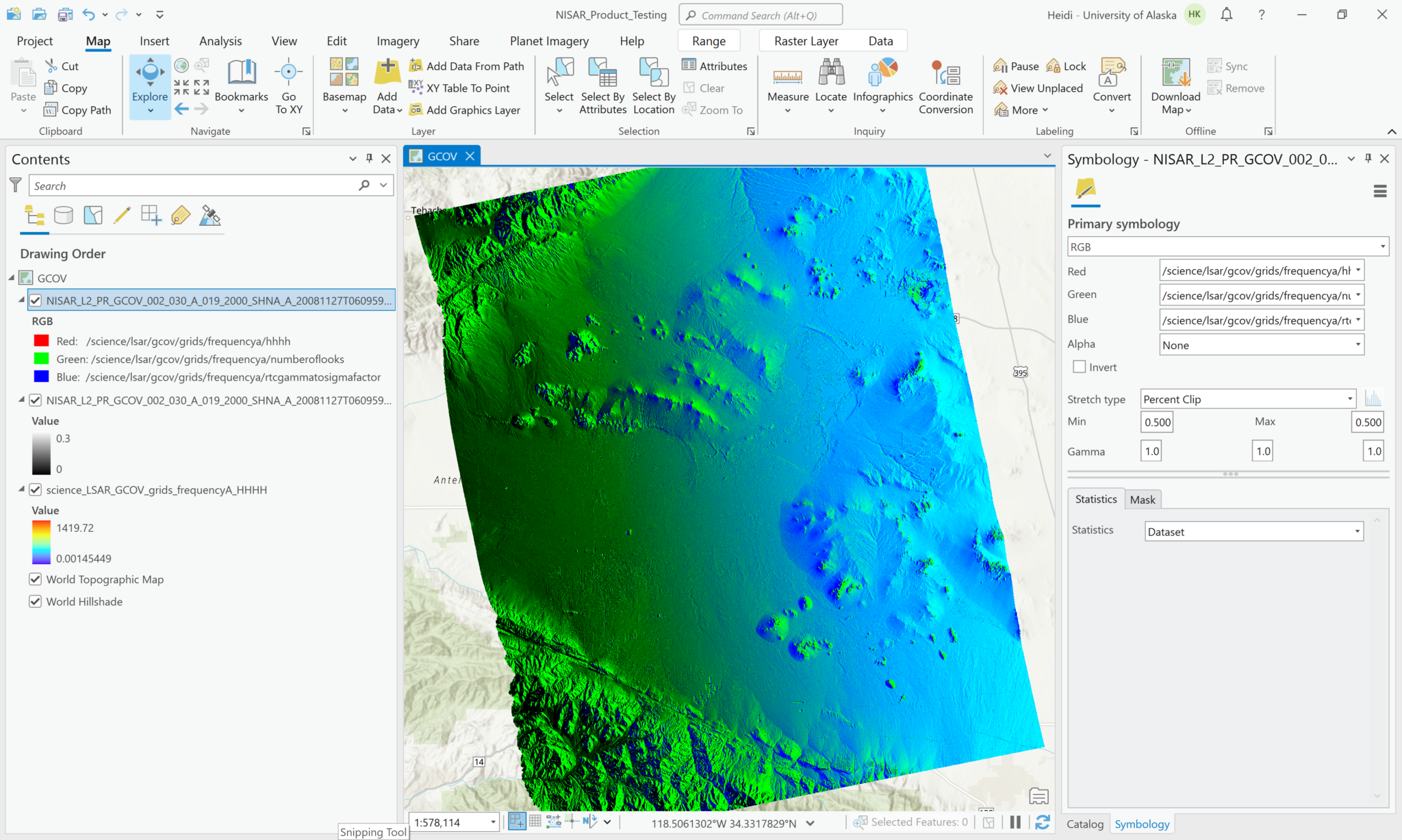
In the example below, the HH backscatter is assigned to the red channel, the number of looks to the green channel, and the rtc gamma to sigma factor to the blue channel. It doesn’t make for a very compelling view, but if you had multiple covariance variables with different polarizations available in the HDF5 file, this approach would be a quick way to display a simple RGB decomposition of the available polarizations.
The sample Geocoded Unwrapped Interferogram (GUNW) data file is:
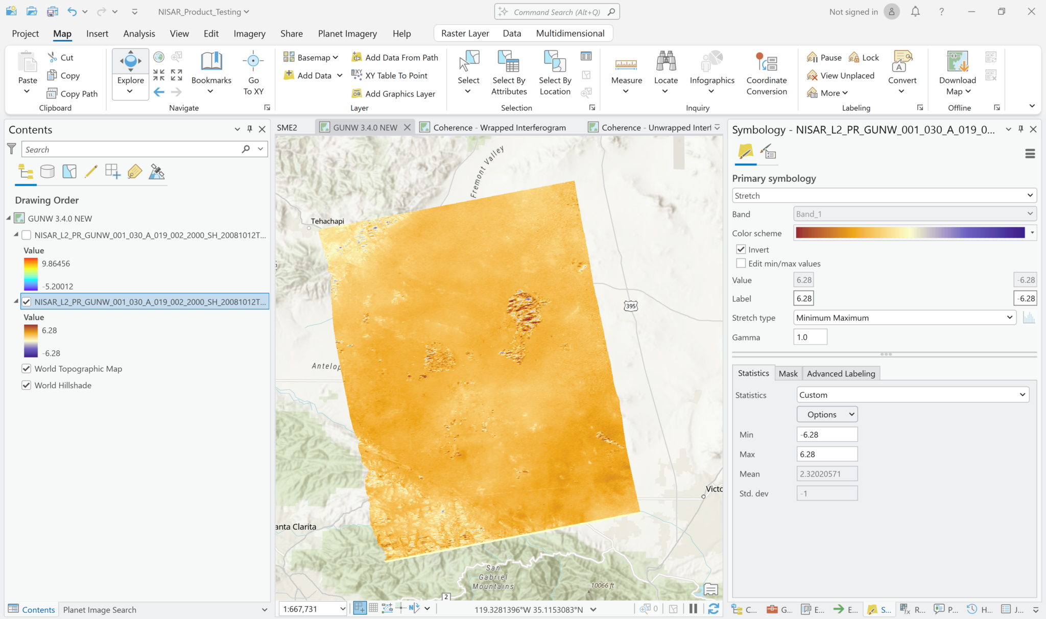
NISAR_L2_PR_GUNW_001_030_A_019_002_2000_SH_20081012T060912_20081012T060924_20081127T061001_20081127T061013_D00402_M_P_J_001.h5
While the product name calls out that the interferograms have been unwrapped, both the wrapped and unwrapped phase difference products are included as variables.
Most of the variables in this file have float or integer pixel types, but the wrapped phase variable has a complex pixel type. ArcGIS can display all of the variables, but refer to the Wrapped Phase section for details on how to appropriately visualize complex datasets. This table describes the pixel types for each variable included in the grids group of the h5 file:
| Variable | Pixel Type |
|---|---|
| /science/LSAR/GUNW/grids/frequencyA/pixelOffsets/HH/alongTrackOffset | 32-bit float |
| /science/LSAR/GUNW/grids/frequencyA/pixelOffsets/HH/correlationSurfacePeak | 32-bit float |
| /science/LSAR/GUNW/grids/frequencyA/pixelOffsets/HH/slantRangeOffset | 32-bit float |
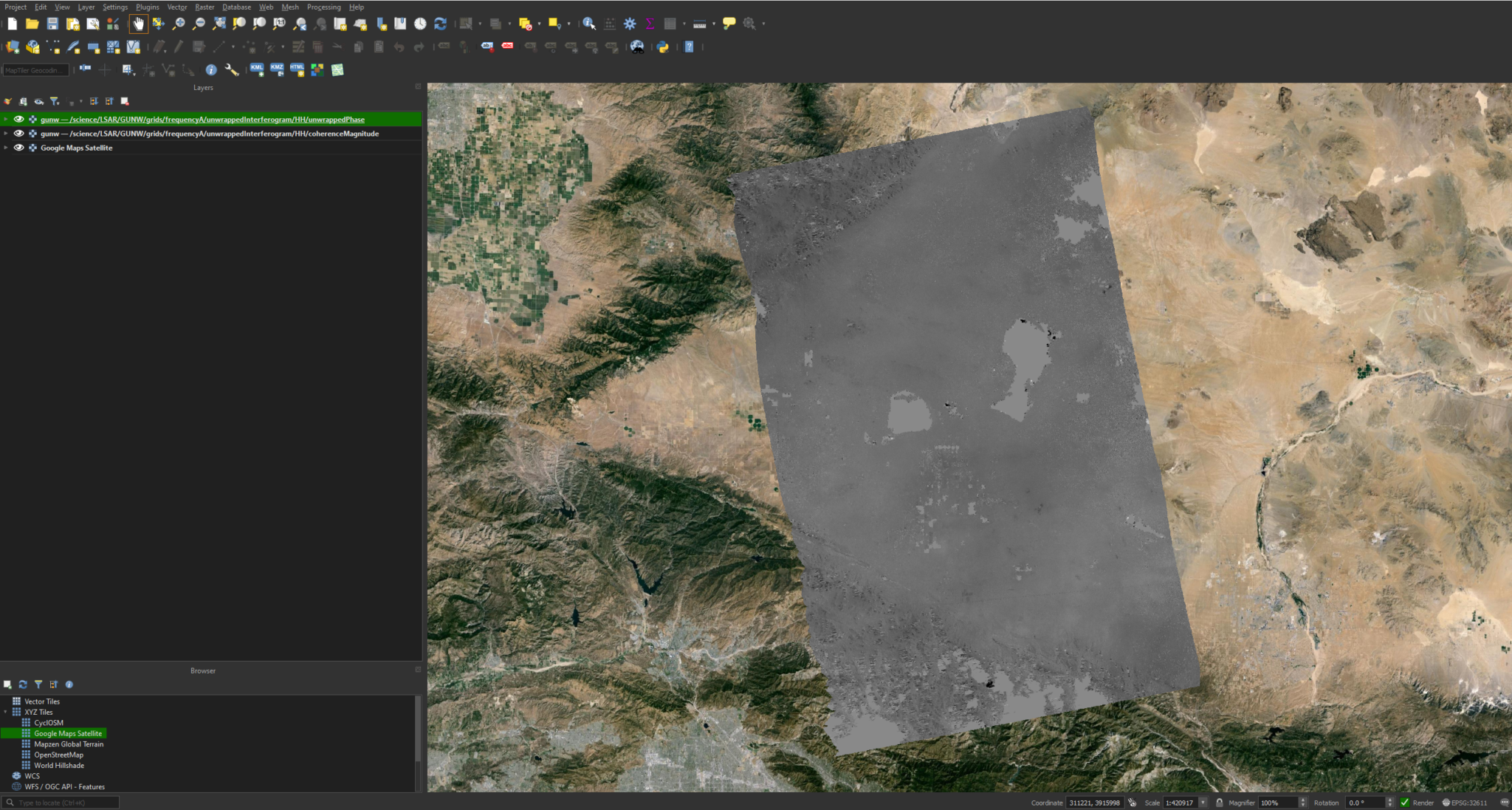
| /science/LSAR/GUNW/grids/frequencyA/unwrappedInterferogram/HH/coherenceMagnitude | 32-bit float |
| /science/LSAR/GUNW/grids/frequencyA/unwrappedInterferogram/HH/connectedComponents | 32-bit unsigned integer |
| /science/LSAR/GUNW/grids/frequencyA/unwrappedInterferogram/HH/ionospherePhaseScreen | 32-bit float |
| /science/LSAR/GUNW/grids/frequencyA/unwrappedInterferogram/HH/ionospherePhaseScreenUncertainty | 32-bit float |
| /science/LSAR/GUNW/grids/frequencyA/unwrappedInterferogram/HH/unwrappedPhase | 32-bit float |
| /science/LSAR/GUNW/grids/frequencyA/unwrappedInterferogram/mask | 8-bit char |
| /science/LSAR/GUNW/grids/frequencyA/wrappedInterferogram/HH/coherenceMagnitude | 32-bit float |
| /science/LSAR/GUNW/grids/frequencyA/wrappedInterferogram/HH/wrappedInterferogram | 64-bit complex |
To learn more about InSAR products in general, including the difference between wrapped and unwrapped phase and the meaning of coherence, refer to ASF’s Exploring Sentinel-1 InSAR tutorial.
Add GUNW Data – Float Format
Any of the variables that are not 64-bit complex can be added to the ArcGIS Pro project using the standard methods. The wrapped interferogram (and any other complex variable) must be added as a Multiband Raster in order to make use of the tools available for extracting phase measurements from the dataset. Refer to the Add Complex Data section for more information.
If you simply drag and drop the GUNW HDF5 file from the Catalog pane into a Map in ArcGIS Pro, it will display the alongTrackOffset variable by default.
The GUNW products include quite a few gridded variables, as listed in the table above. There are also many metadata variables from the /science/LSAR/GUNW/metadata/radarGrid/ path that can be visualized in the map, as well.
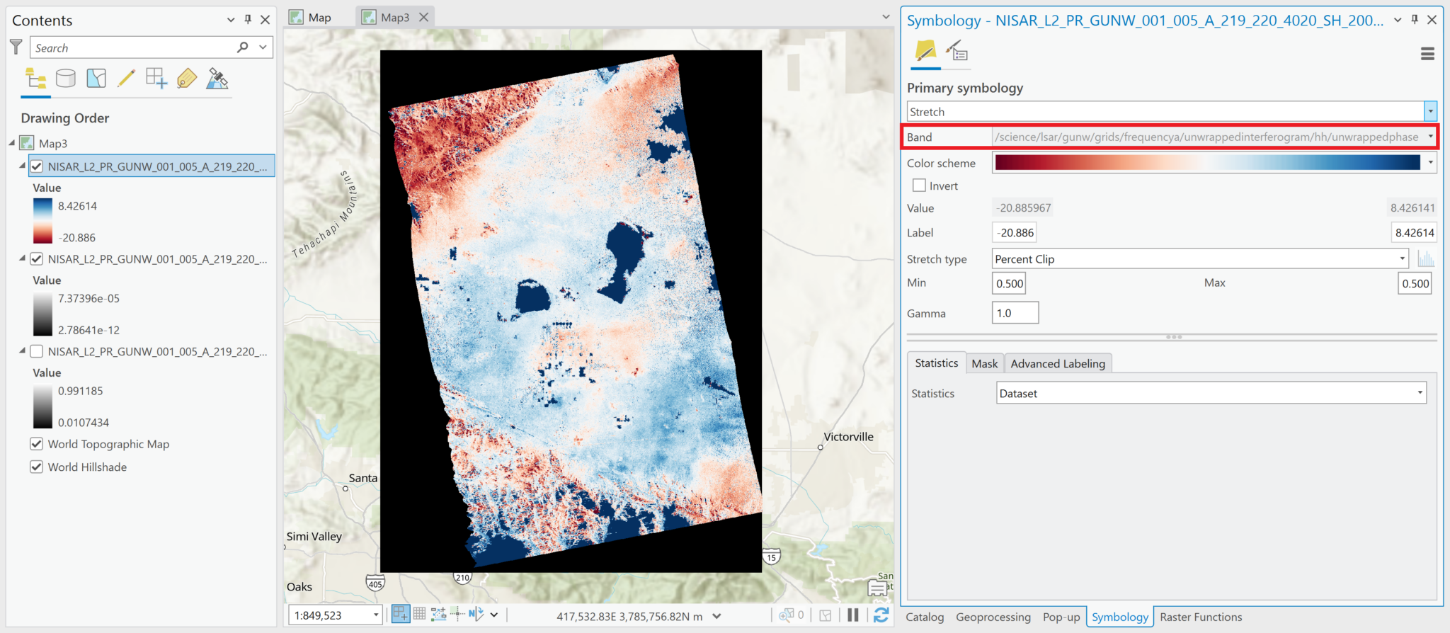
The most common variables to visualize are the unwrapped phase, the wrapped interferogram, and the coherence magnitude (note that coherence variables are available based on both the wrapped and unwrapped interferograms).
Note that there are limitations for working with the wrapped interferogram if it is added as a multidimensional raster layer. It will display the Amplitude values by default, but you will not be able to use the Complex raster function to access the Phase values. Refer to the Add Complex Data and Wrapped Phase sections for more information.
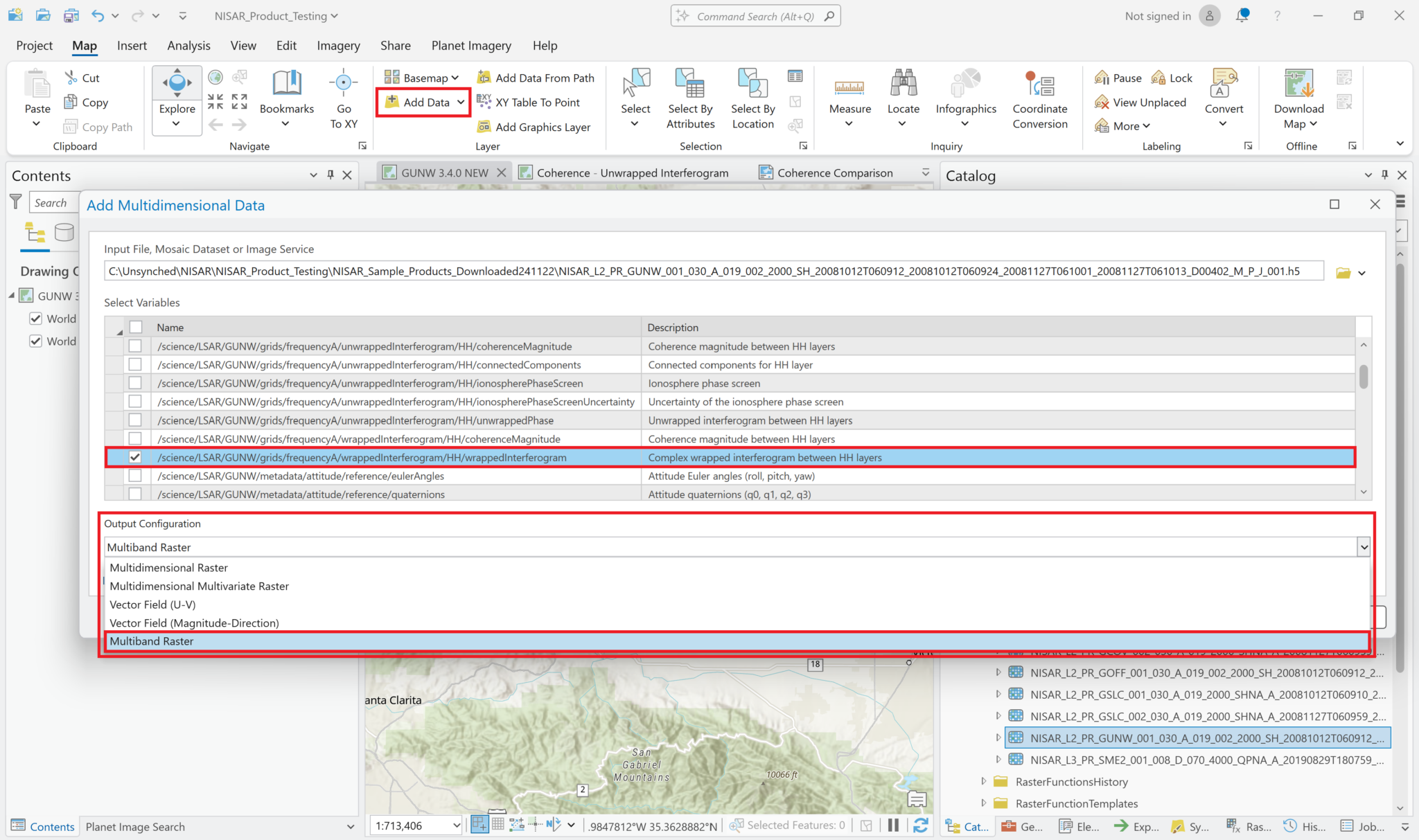
Add Complex Data
For variables with 64-bit complex pixel values, such as the wrapped interferogram, you must add the data as a Multiband Raster layer in order to allow for the correct extraction of the phase measurements. The Complex raster function, described in the Wrapped Phase section does not function properly if the variable was added as a Multidimensional Raster layer.
Use the same Add Multidimensional Data workflow to navigate to the HDF5 file, but after selecting the complex variable, select Multiband Raster from the dropdown menu for the Output Configuration.
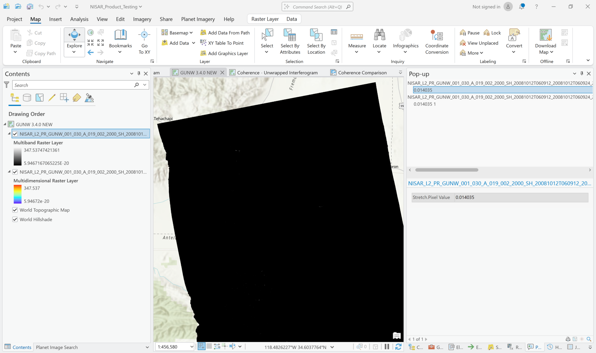
By default, the pixel values displayed when the image is added will indicate Amplitude. If you add the variable using the Multidimensional Raster output configuration, Pro will also display the Amplitude values by default, but you will not be able to extract the Phase values.
Note in the image below that the pixel values are the same in the default visualization of the wrapped interferogram, regardless of whether it was added as a Multiband Raster or Multidimensional Raster layer.
By default, Multiband Raster layers are displayed in grayscale and Multidimensional Raster layers use a color scheme.
Visualize GUNW Products
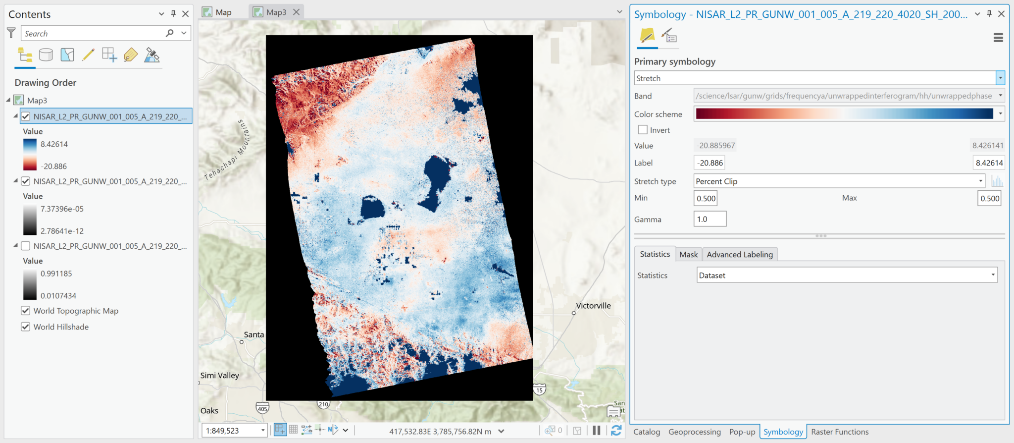
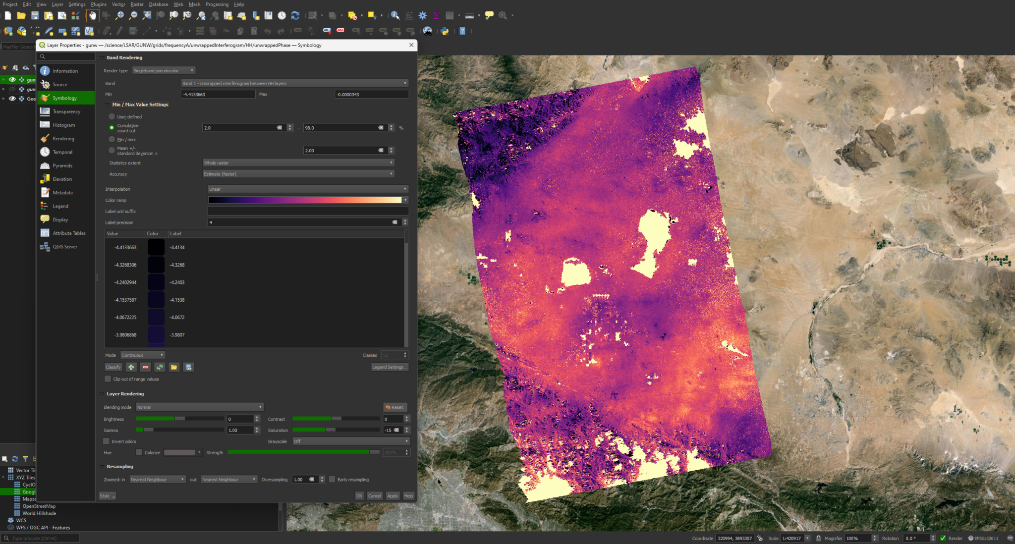
You can adjust the symbology of most NISAR GUNW variables as you would any other raster, with the majority of these adjustments involving the stretch characteristics. There are some additional considerations to keep in mind when visualizing the wrapped phase, however, so we’ll start with that.
Wrapped Phase
The wrapped phase variable has a complex pixel type, containing both real and imaginary components that can be used to calculate either the amplitude or the phase values for the dataset. When looking at an interferogram to detect and quantify surface deformation, we’re interested in differences in phase rather than in amplitude.
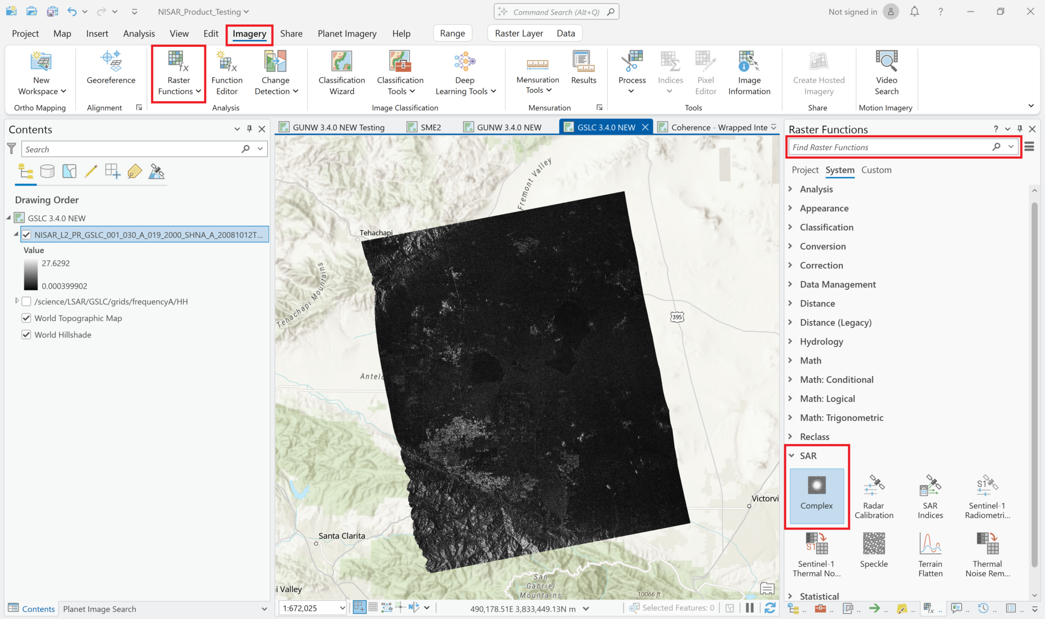
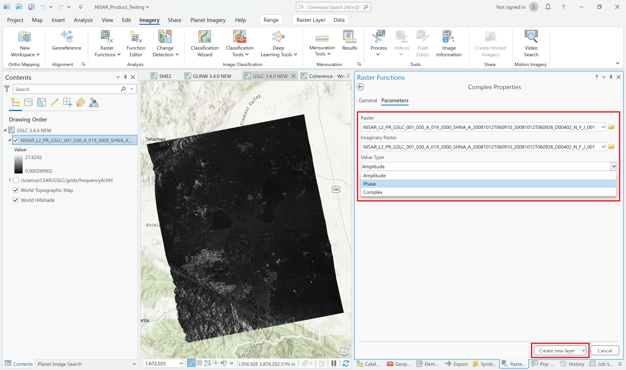
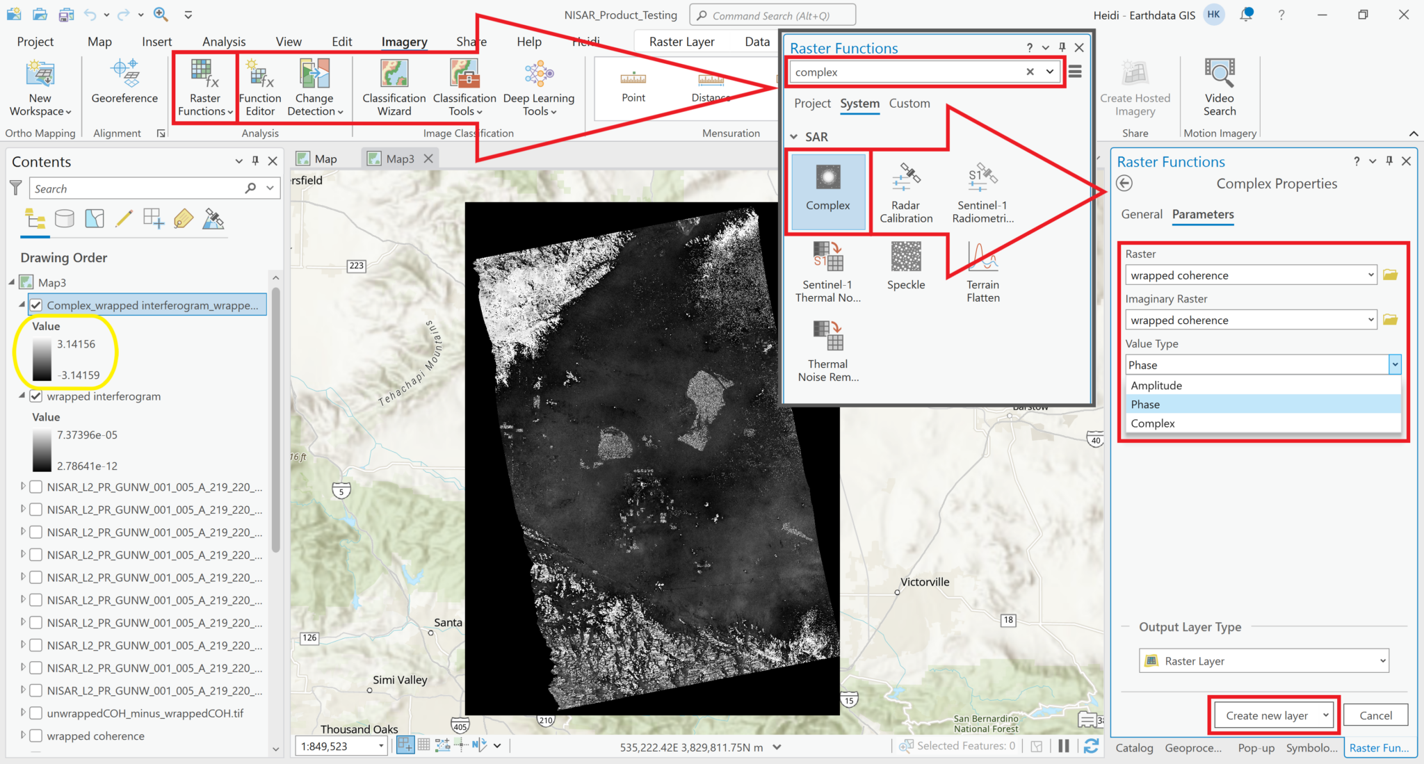
ArcGIS Pro provides a ‘Complex’ raster function, which can be used to display the phase values instead of amplitude values. It is included in the SAR section of the raster functions panel in ArcGIS Pro. This raster function requires that the variable be added as a Multiband Raster rather than a Multidimensional Raster layer.
- Add the wrapped interferogram variable to the map, ensuring that you set the
Output ConfigurationtoMultiband Raster, as described in the Add Complex Data section. - From the
Imagerymenu, selectRaster Functionsto open the Raster Functions panel - Type
Complexin the search bar at the top of the Raster Functional panel, and click on theComplexraster function - Select the wrapped interferogram layer in both the Raster and the Imaginary Raster fields
- Select
Phasefrom theValue Typedrop-down menu - Click the
Create New Layerbutton to display a layer showing the phase difference values of the wrapped interferogram (or use the arrow next to theCreate New Layertext to select the option to save the output as a stand-alone raster).
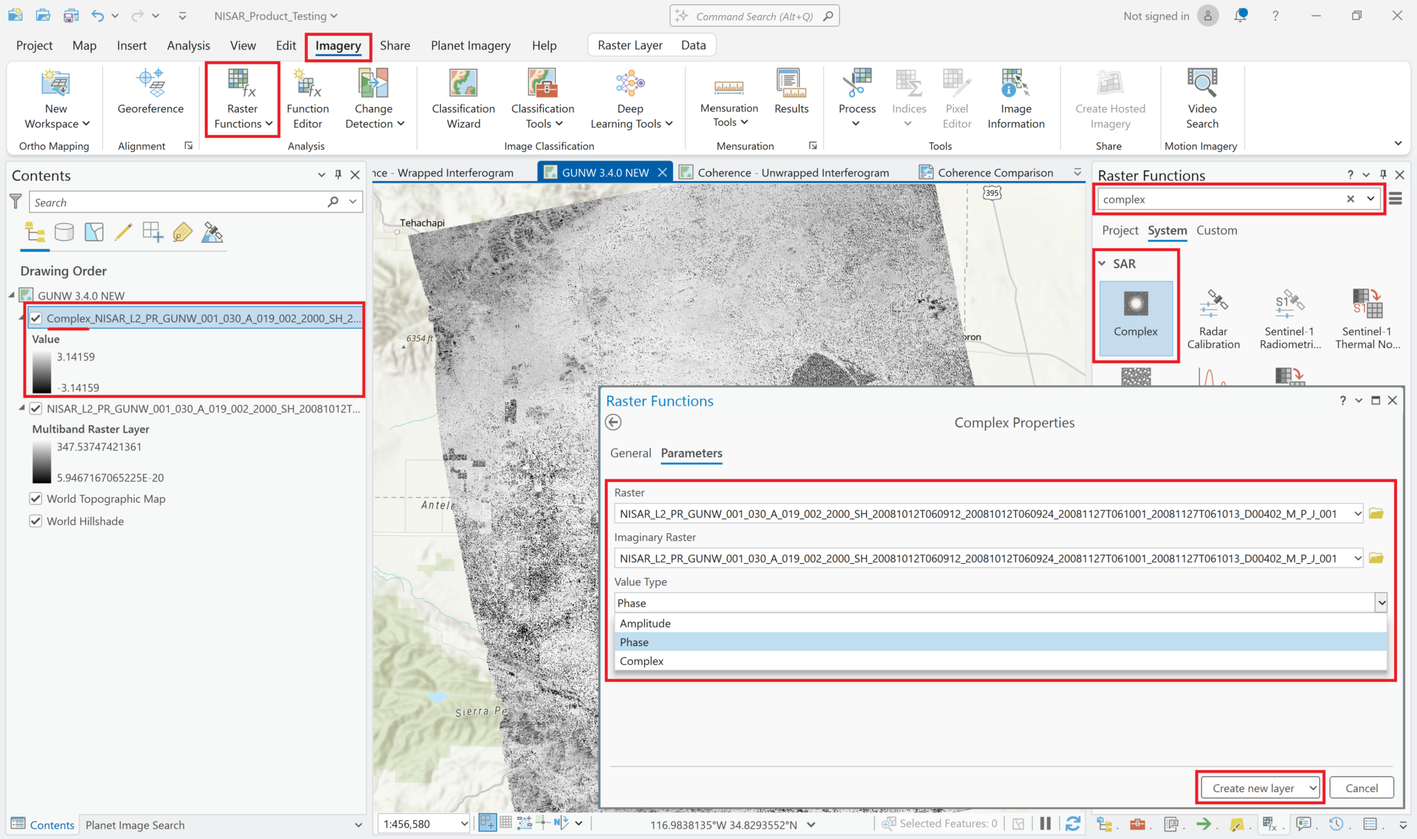
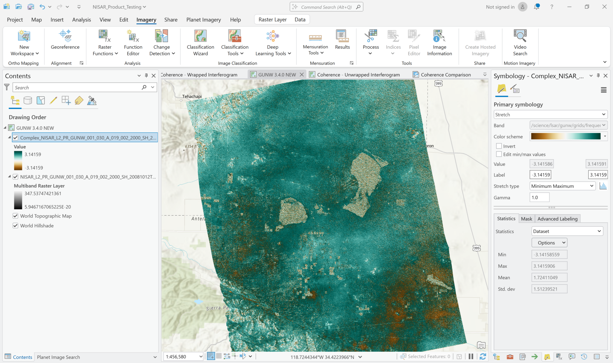
The values displayed in the image now range from -pi to pi, which is what we would expect for phase measurements in a wrapped interferogram.
Note that the phase layer is a virtual raster that is displayed on-the-fly in your project, but you can export the layer as a stand-alone raster if you would like to save it for future use in other applications.
It may be helpful to adjust the symbology so that the stretch displays the full range of values (Minimum-Maximum). Applying a color scheme where 0 values have a neutral color may also help to indicate the sign and magnitude of the phase differences between the two acquisitions.
Unwrapped Phase
Phase unwrapping converts the wrapped phase values, which are constrained to a range of -3.14 to 3.14 radians, to a continuous range of consecutive multiples of 2π radians. The output values are no longer complex values, but are 32-bit float values with units of radians. You can treat the unwrapped phase variable like any other multidimensional raster. Note that the pop-up indicates that the pixel values are in radians.
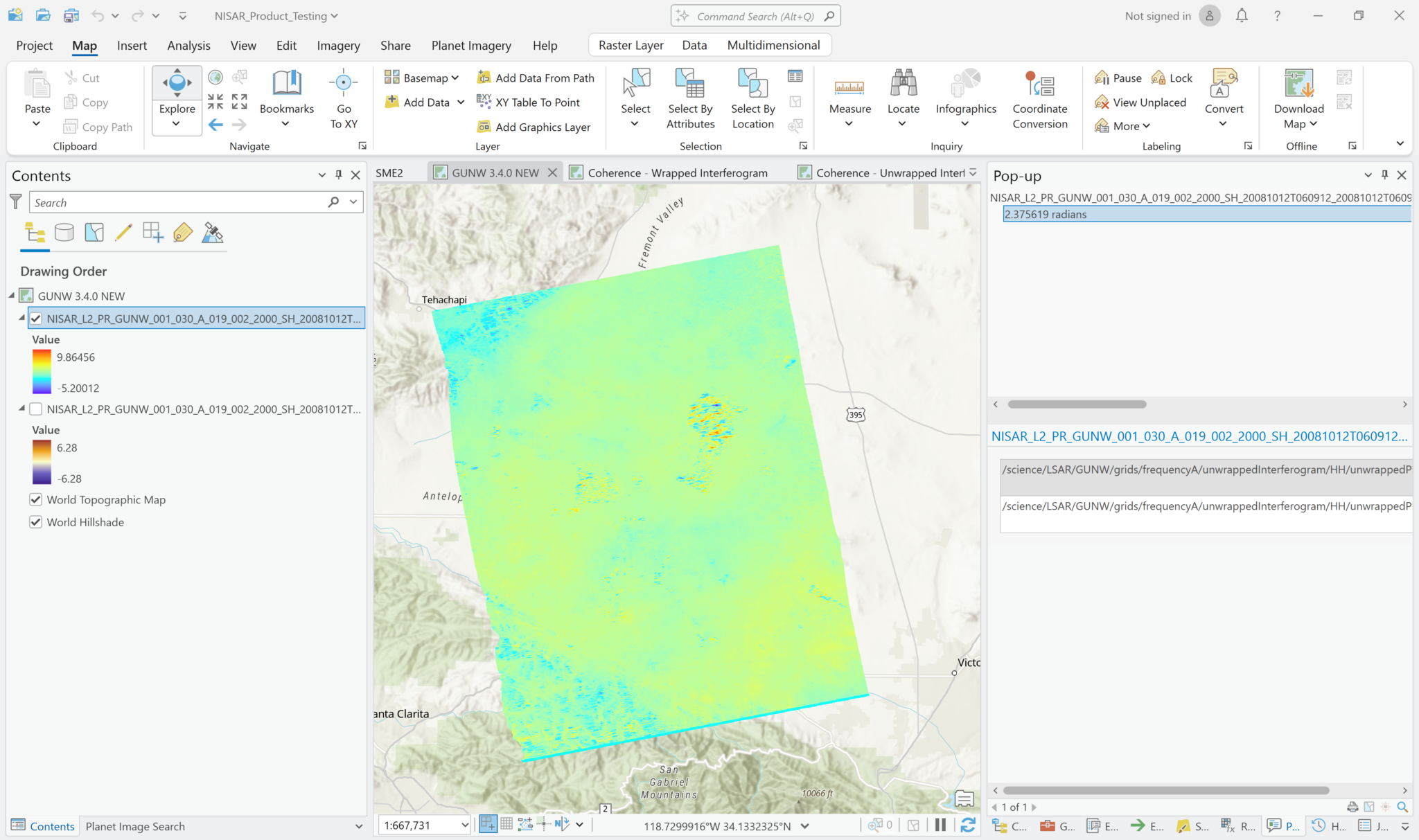
Adjust the symbology as desired to highlight the information you want to see. To get a sense of the overall direction of phase difference, try setting custom Minimum-Maximum values that are equal in magnitude in the positive and negative directions and apply a color scheme with a neutral color in the middle.
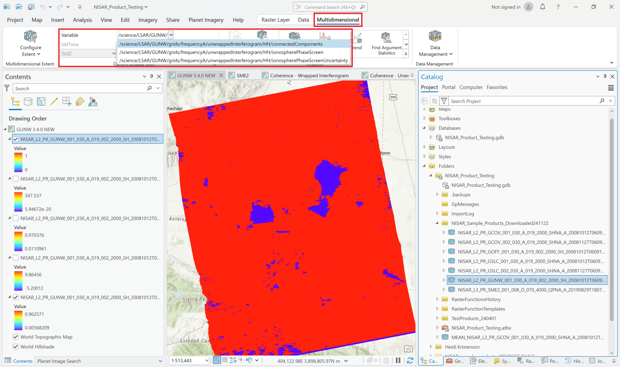
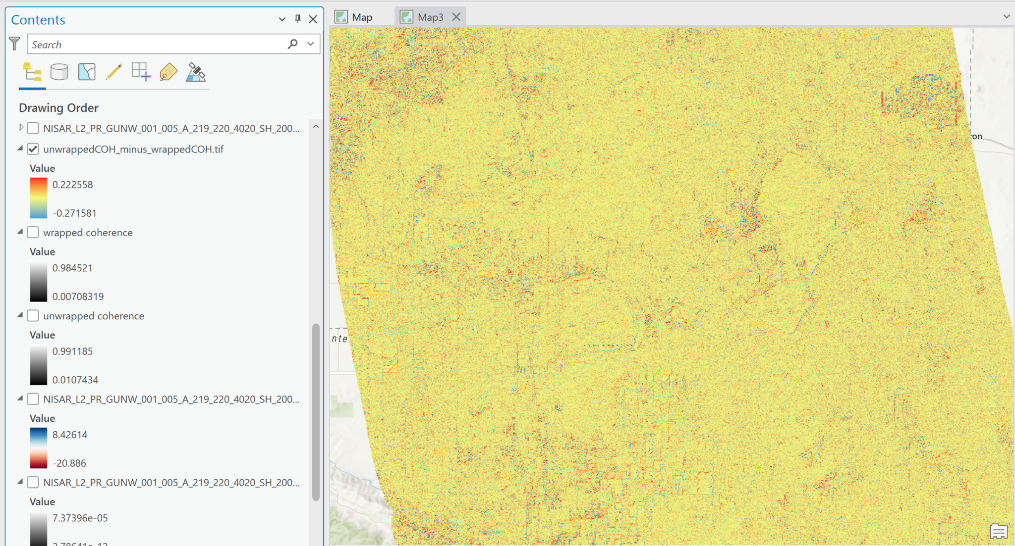
Coherence Products
There are two different coherence variables included in the GUNW product: wrapped and unwrapped coherence. Both variables have pixel values that range between 0 and 1, with values closer to 0 indicating low coherence and values closer to 1 indicating high coherence.
The key difference between these two variables is that there is multilooking applied to the unwrapped coherence product. While this decreases the resolution of the data, it can make for a more useful visualization of the overall coherence patterns.
In the comparison below, the wrapped and unwrapped coherence products are displayed both zoomed in to the level where individual pixels are visible (top images) and zoomed out to nearly the full extent of the image.
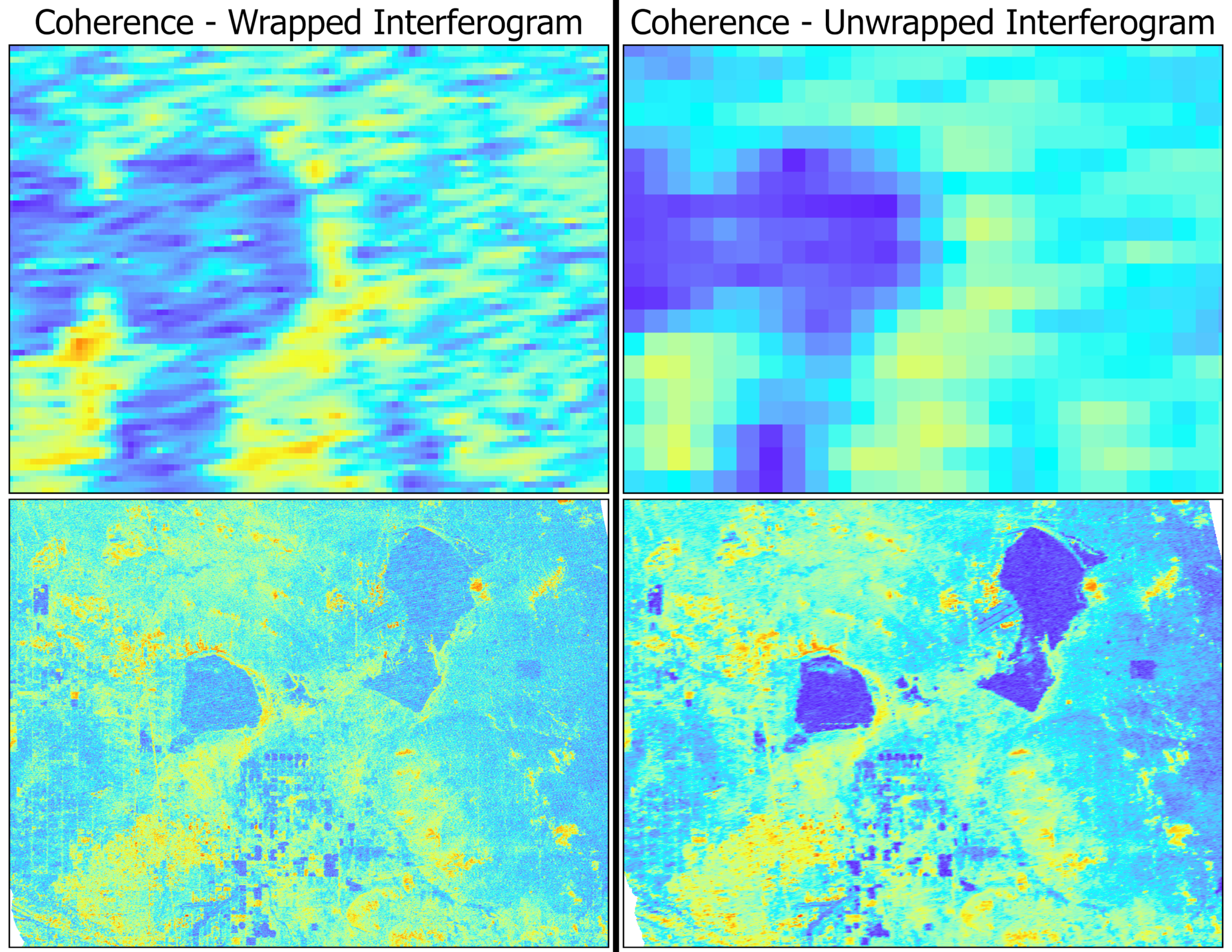
While the wrapped coherence image may provide a more detailed representation, especially when looking at very small individual areas, the unwrapped coherence gives a stronger indication of areas with very low coherence (such as lakes and agricultural fields) and very high coherence (urban areas and regions with little vegetation).
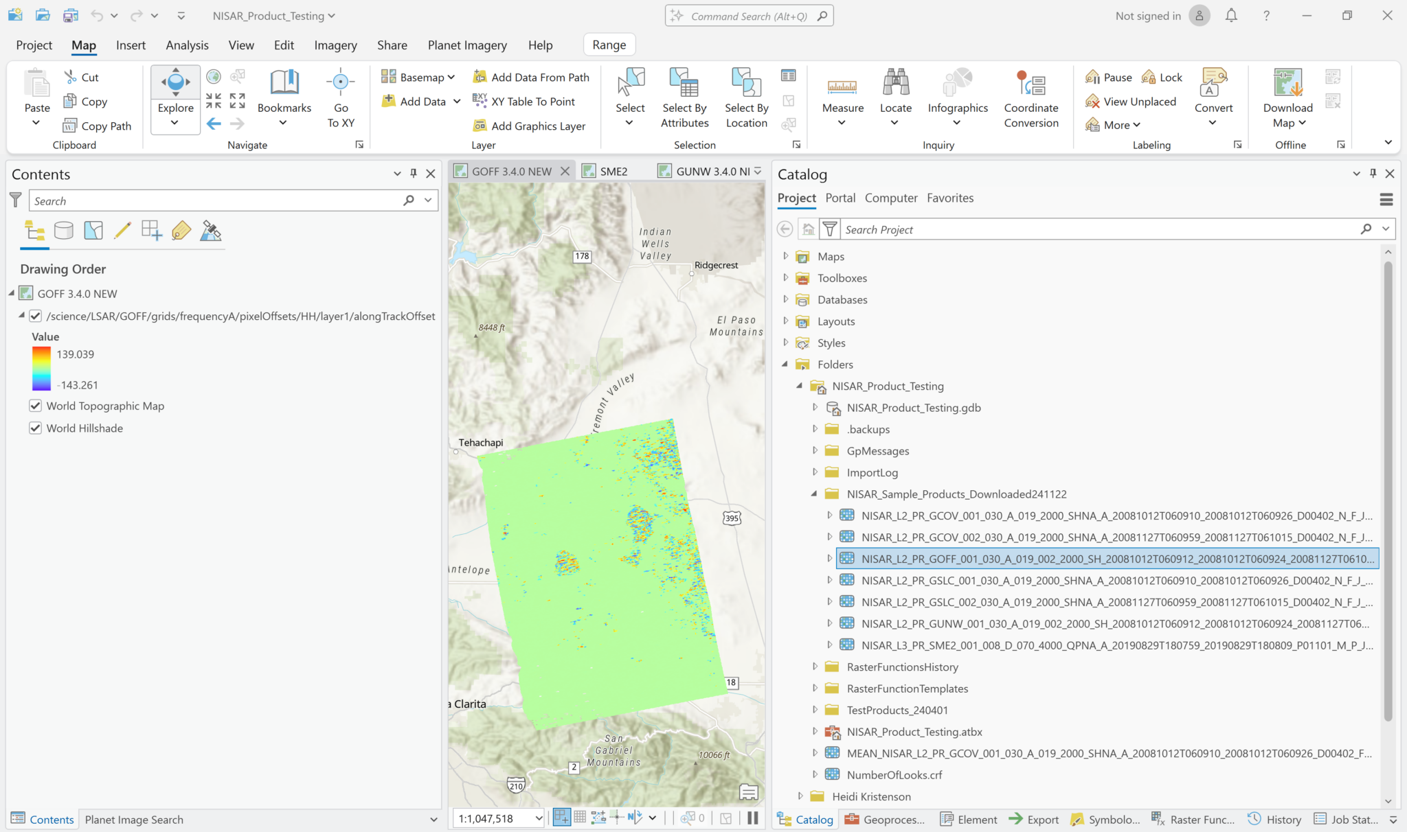
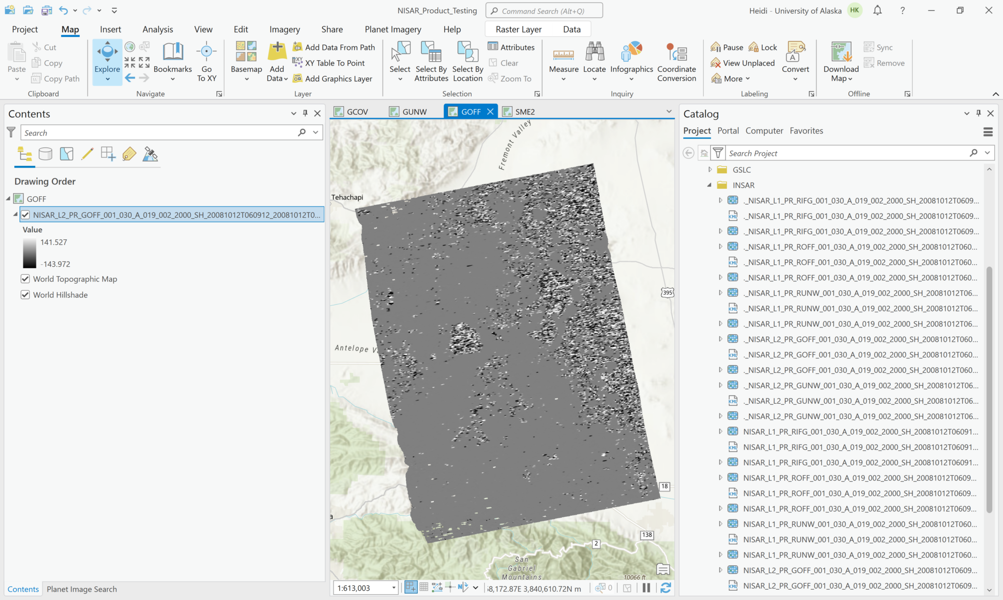
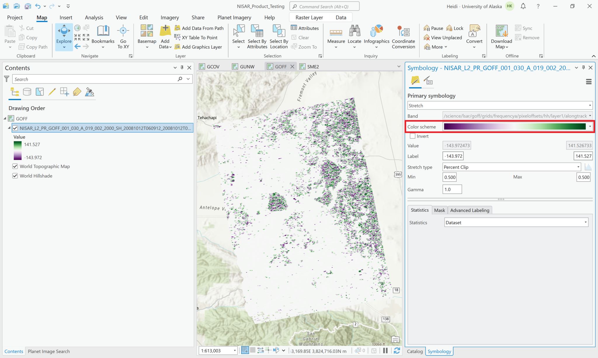
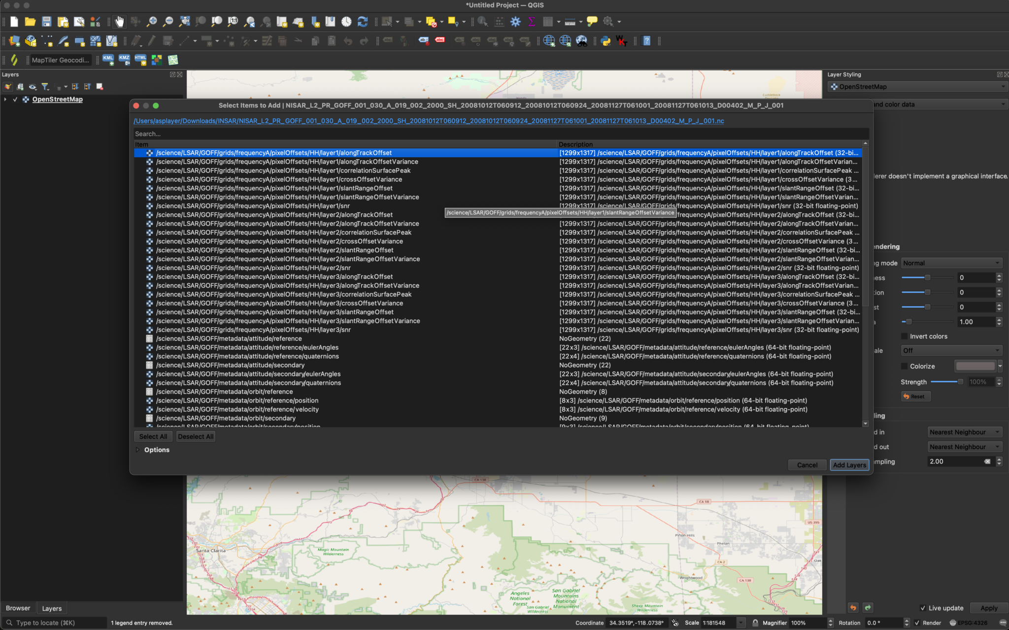
The sample Geocoded Offset (GOFF) data file is:
NISAR_L2_PR_GOFF_001_030_A_019_002_2000_SH_20081012T060912_20081012T060924_20081127T061001_20081127T061013_D00402_M_P_J_001.h5
The approach used in the GOFF products is often called Pixel Tracking.
There are 21 variables included in the grid group, seven variables for each of three different layers, generated with different window sizes. They are all 32-bit float datasets. Variables from this product can be added using any of the standard methods, and visualized as you would any other raster.
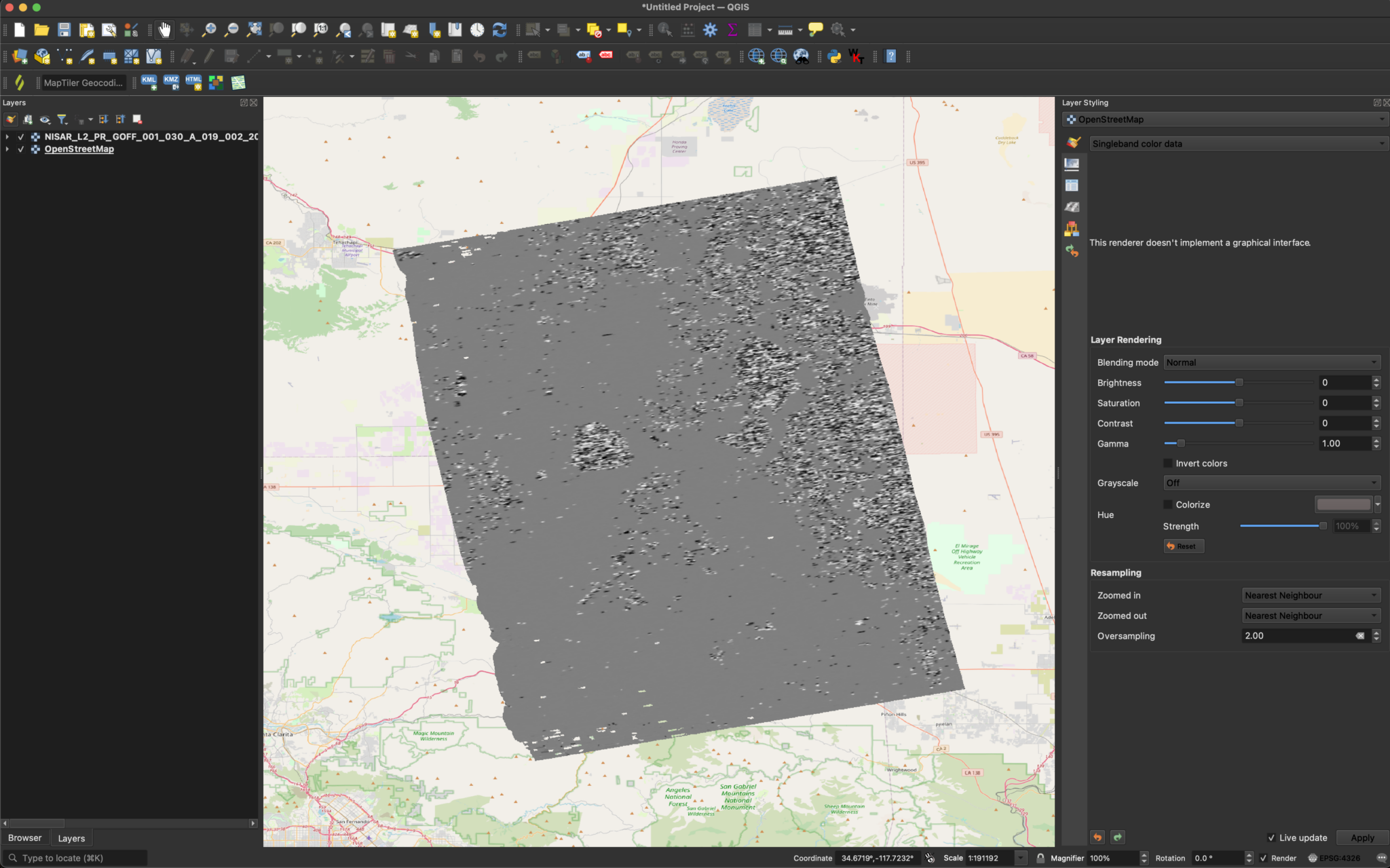
If you drag and drop the GOFF HDF5 product from the Catalog pane to the map, it will display the /science/LSAR/GOFF/grids/frequencyA/pixelOffsets/HH/layer1/alongTrackOffset variable.
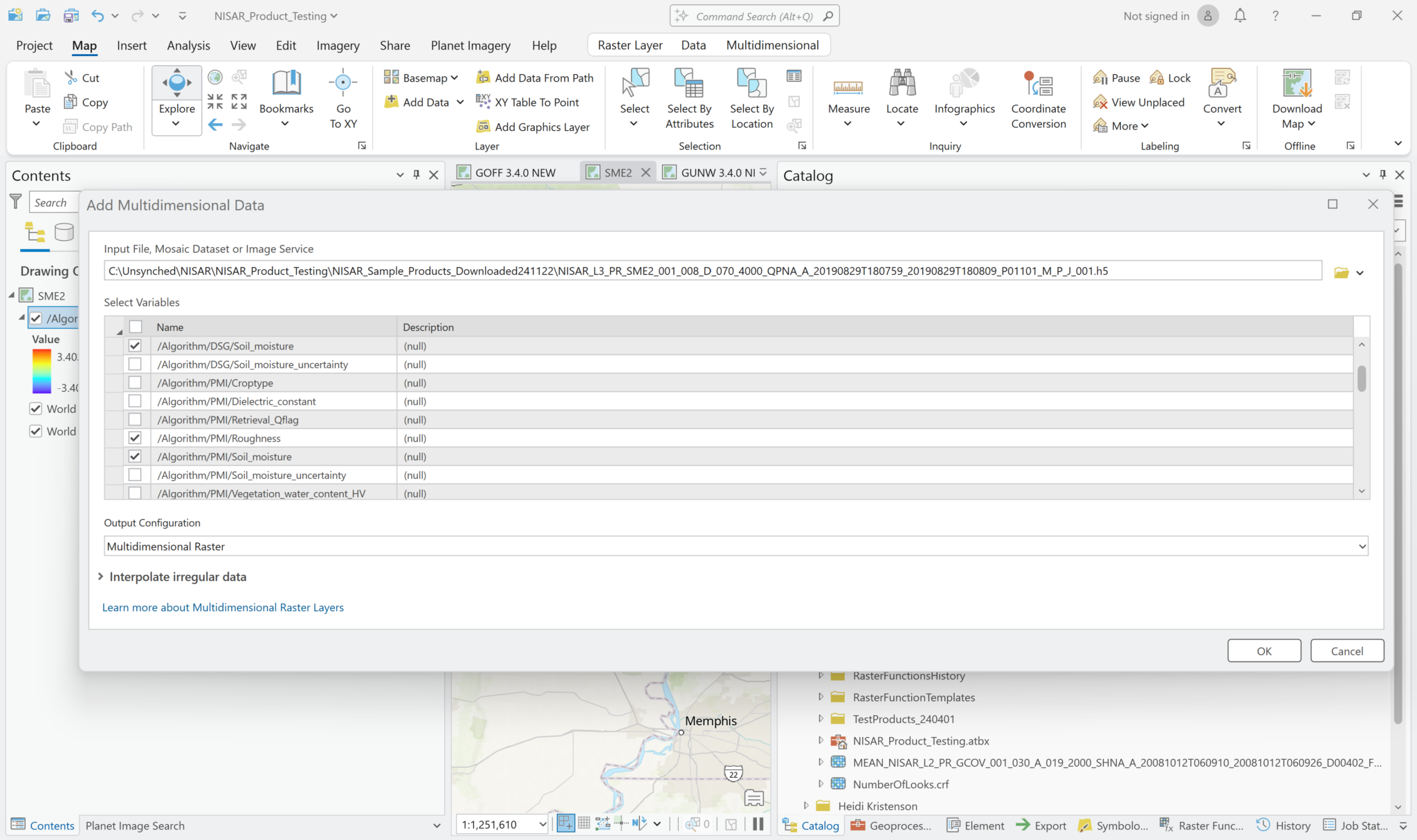
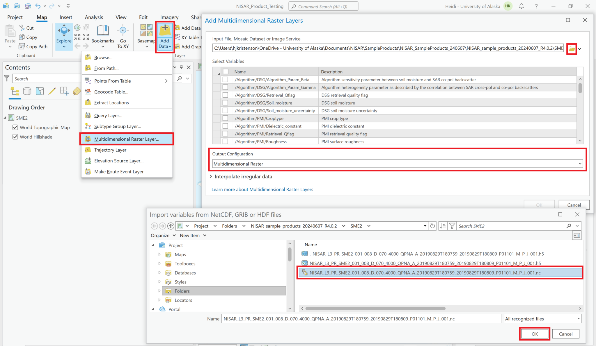
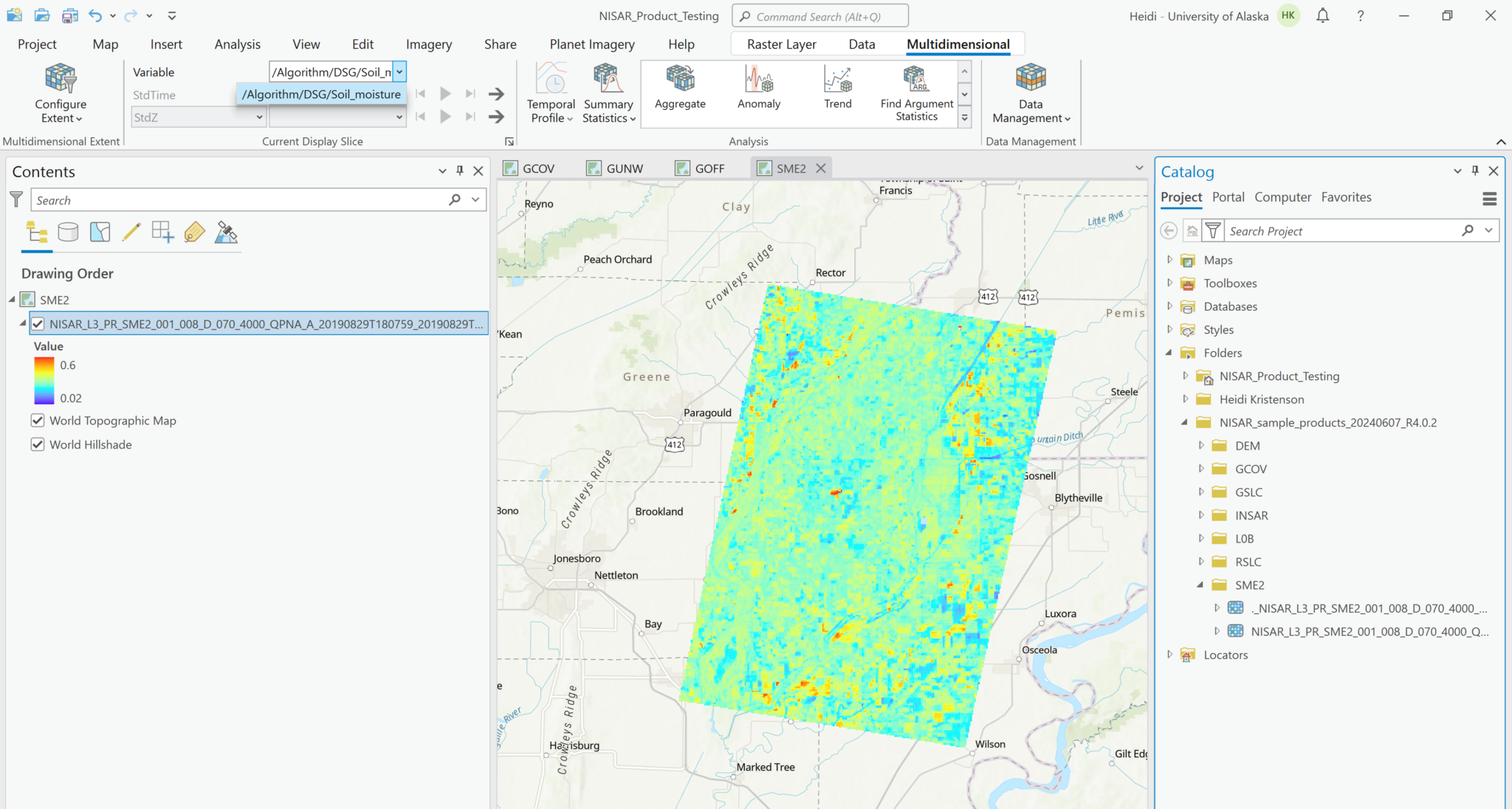
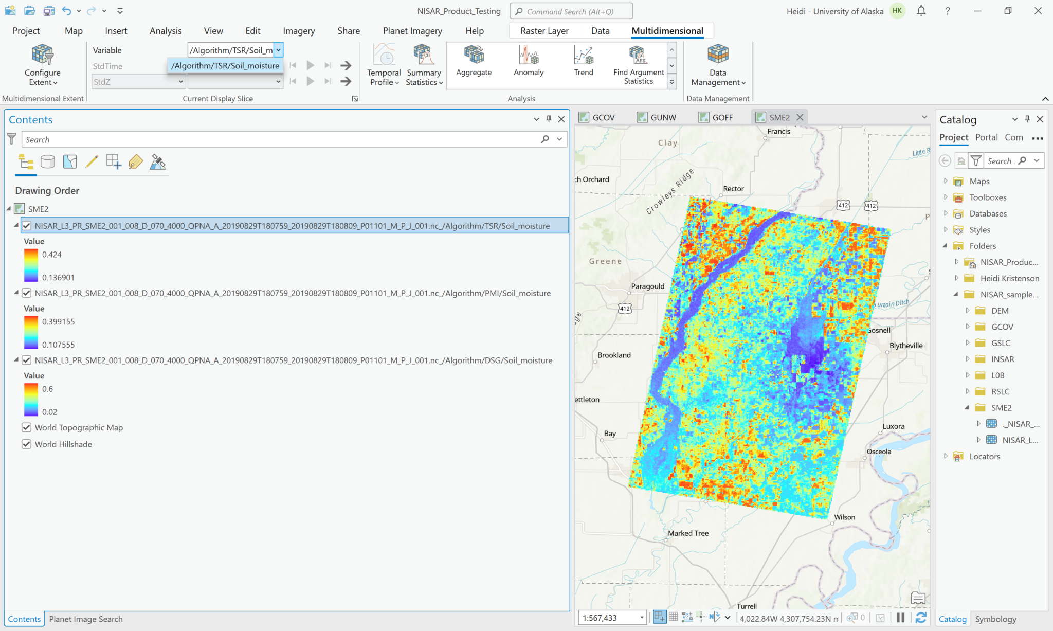
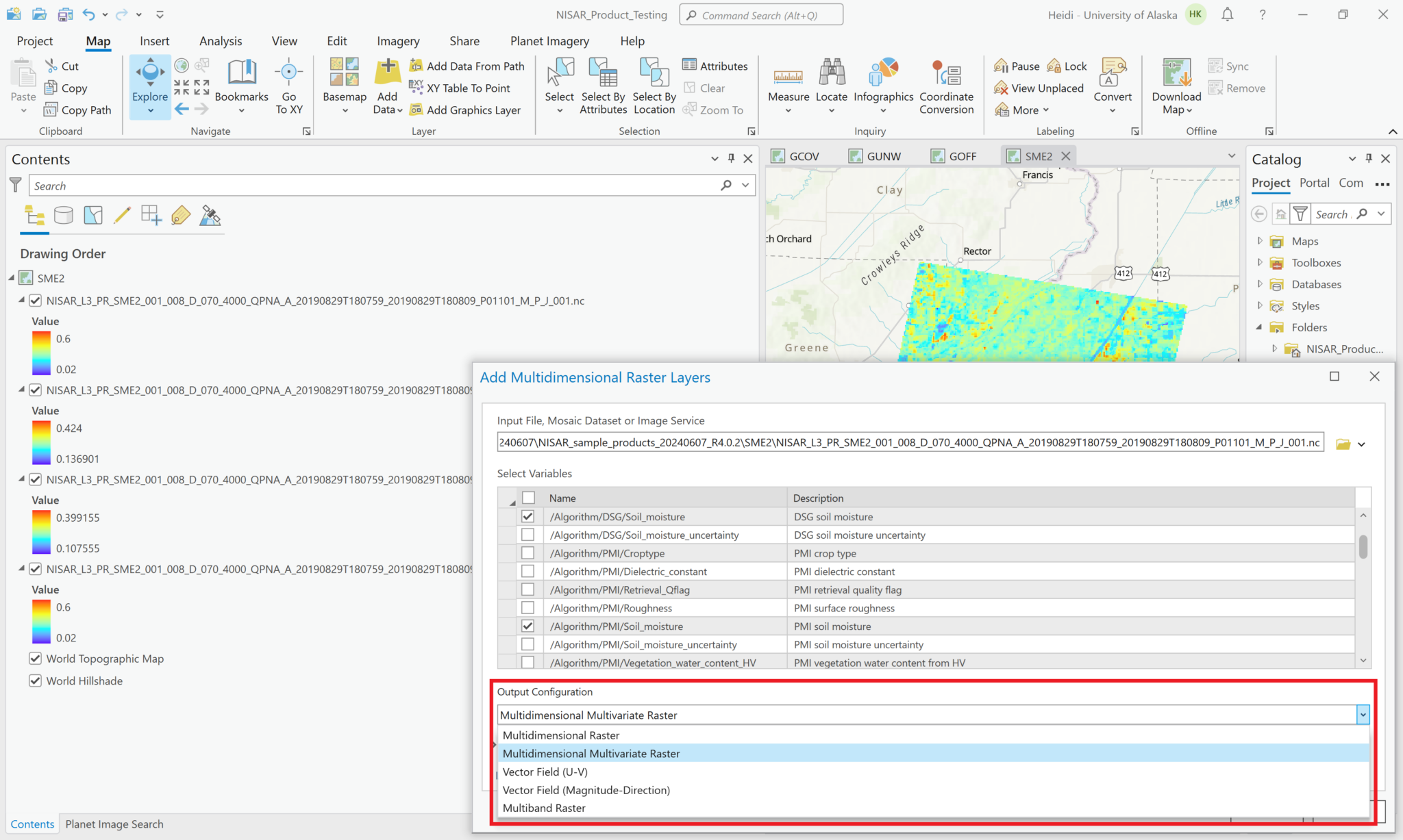
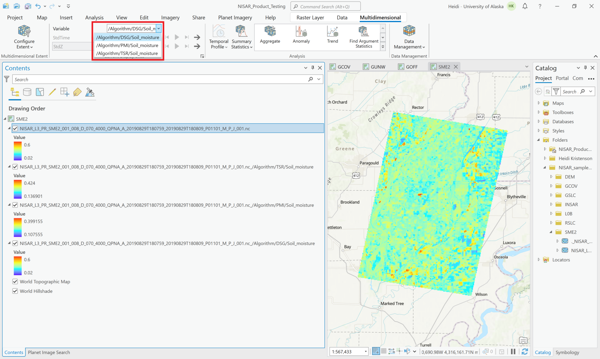
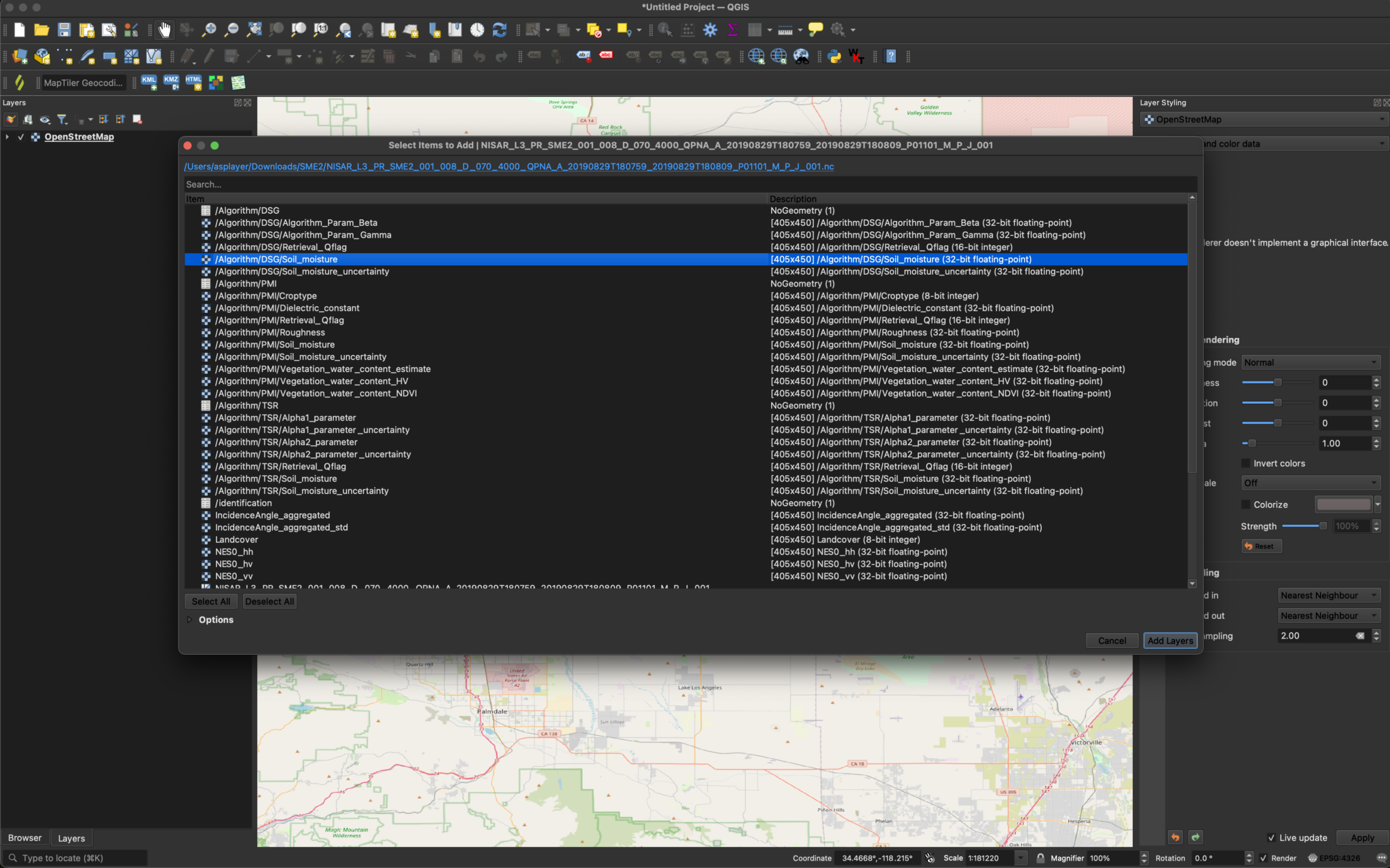
There is one sample Soil Moisture (SME2) product:
NISAR_L3_PR_SME2_001_008_D_070_4000_QPNA_A_20190829T180759_20190829T180809_P01101_M_P_J_001.h5
Note that the product linked on the JPL site does not appear to be the most recent iteration of the test data. The key issues are:
- The variable descriptions are blank
- NoData pixels are assigned a value of -9999, which complicates visualization of the data
You can still use any of the standard methods to add the variables to your project, however.
If you use the drag-and-drop method to add the file, the /Algorithm/DSG/Algorithm_Param_Beta variable will be added by default, which is not generally of interest to most users.
There are three different variables containing soil moisture data: DSG (Disaggregated), TSR (Time Series Rates), and PMI (Physical Model Inversion). Use any of the standard methods to add the desired variables to your map.
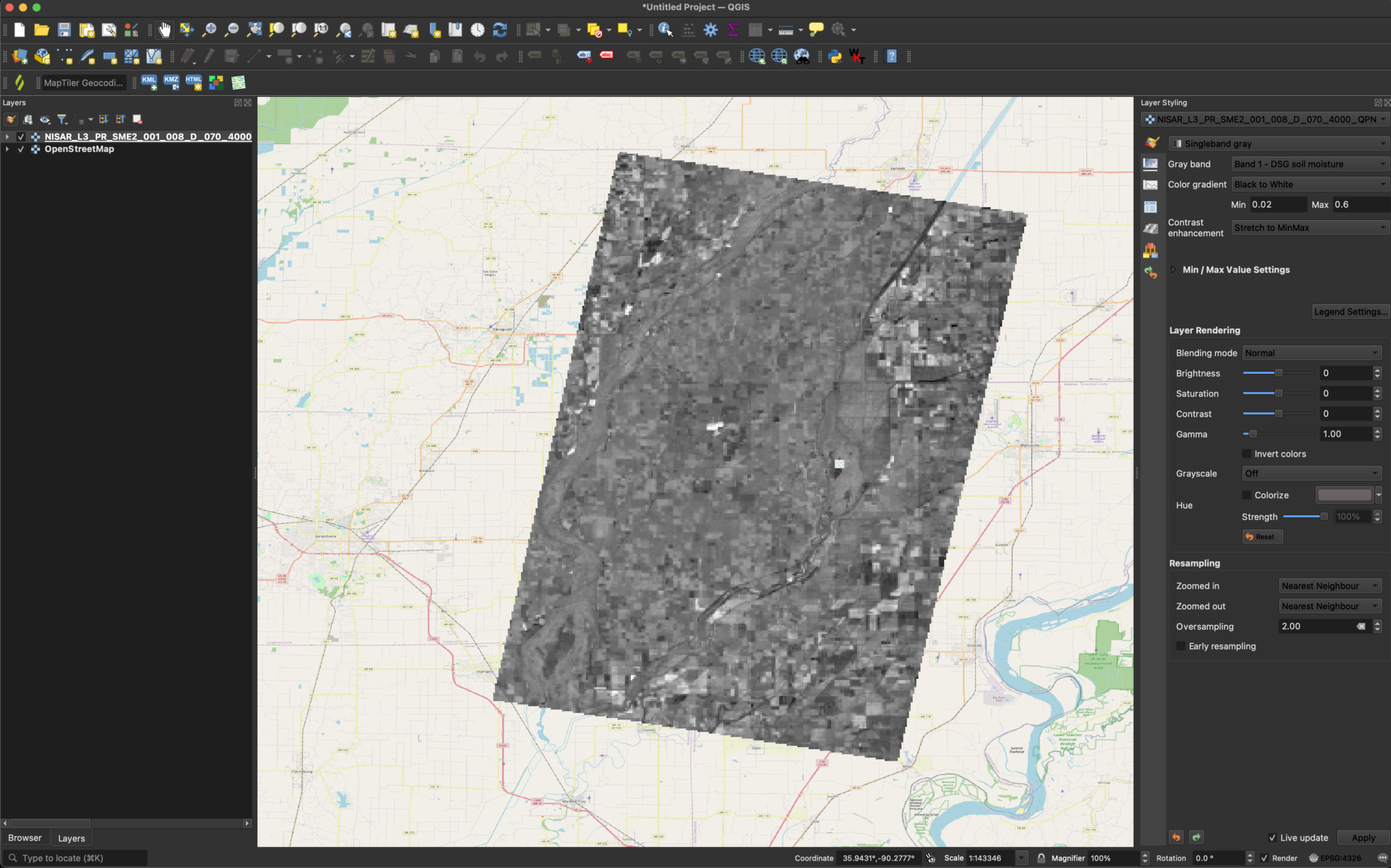
Visualizing SME2 Dta
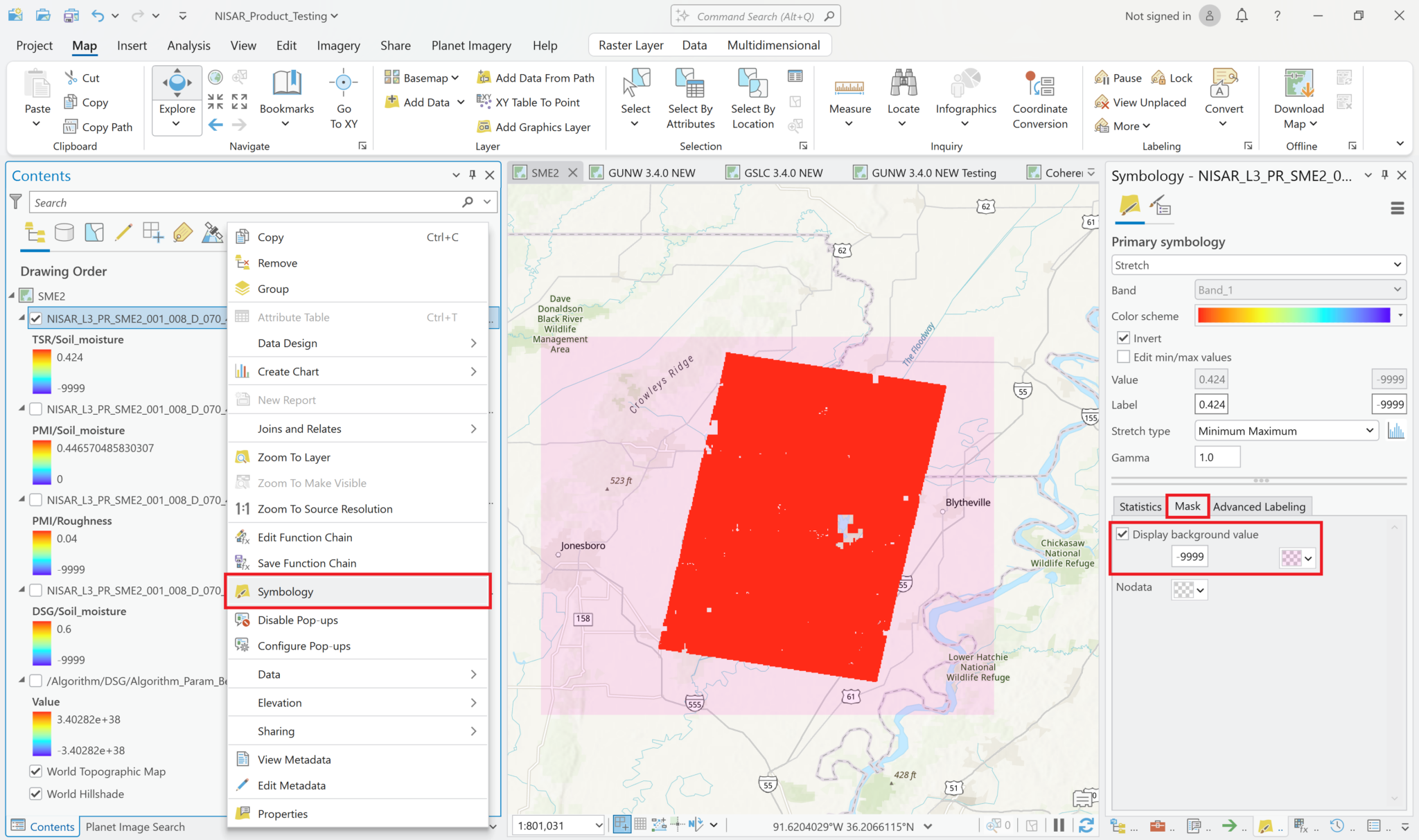
The sample product currently available from the JPL website uses the value -9999 to indicate NoData.
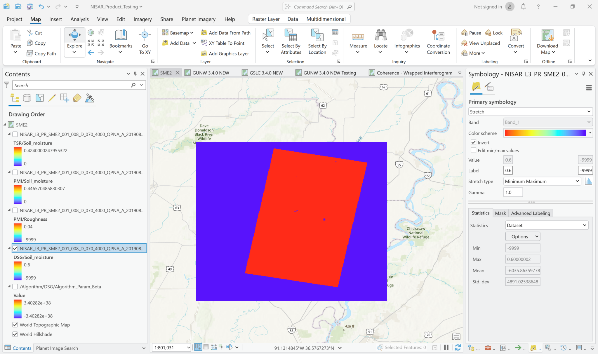
This requires some adjustments to the symbology settings before you can display the data with a meaningful stretch applied.
To adjust the visualization to exclude the -9999 values from the grayscale and treat them as background pixels:
- Right-click on the soil moisture layer, and select
Symbology - Click the
Masktab, check the box toDisplay background value - By default, the background is transparent
- If you want to see the extent of the padding pixels, you can select a color (the illustration used pink)
- Once a color has been selected, click on the color swatch again and select ‘Color Properties’, where you can apply a transparency value if desired (the illustration used 90%)
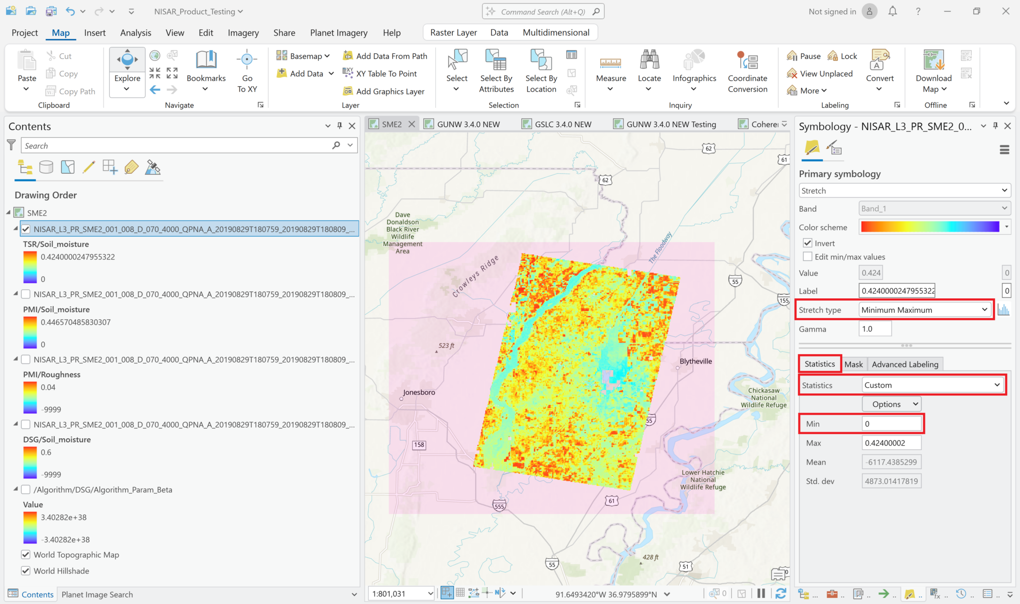
- Change the
Stretch typeto Minimum-Maximum - Select the
Statisticstab - Use the drop-down menu to set the Statistics field to
Custom - Change the value in the Minimum field from
-9999to0and press the tab button to update the scalebar label
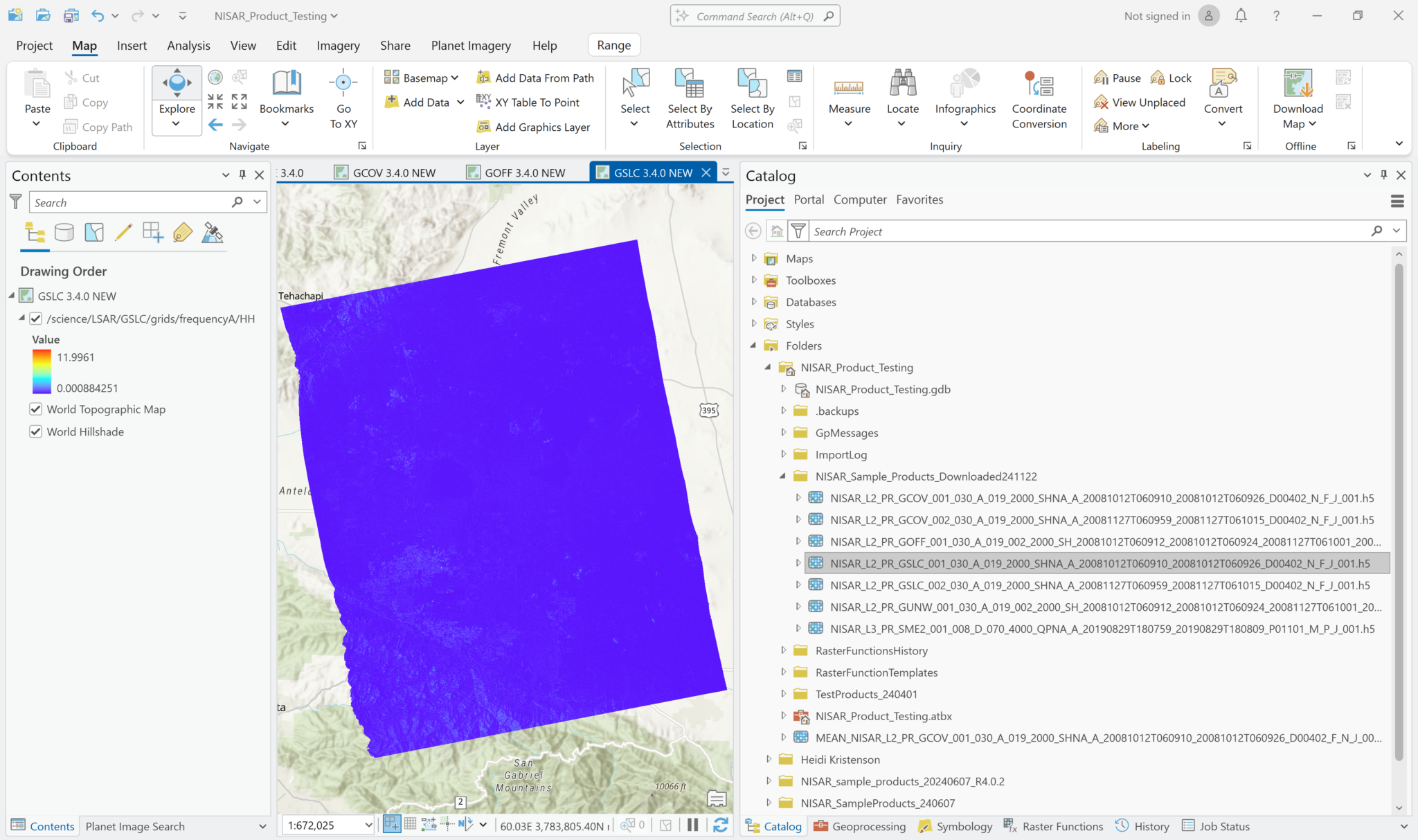
There are two sample Geocoded Single-Look Complex (GSLC) products available, one for each of the acquisitions used in other sample products that require imagery pairs:
NISAR_L2_PR_GSLC_001_030_A_019_2000_SHNA_A_20081012T060910_20081012T060926_D00402_F_N_J_001.h5
NISAR_L2_PR_GSLC_002_030_A_019_2000_SHNA_A_20081127T060959_20081127T061015_D00402_F_N_J_001.h5
The illustrations in this section use the acquisition from October 12, 2008. Note that the data used to create these sample products are from JAXA’s PALSAR sensor, which also operates in the L band, but the product has a smaller footprint than the NISAR acquisitions.
Add GSLC Data
As with the wrapped phase variable in the GUNW products, the SLC variables in the GSLC are in complex data format. While you can add these variables using the Drag and Drop or Add Multidimensional Raster approaches, these methods will display the Amplitude measurements by default, and you will not have access to the phase measurements.
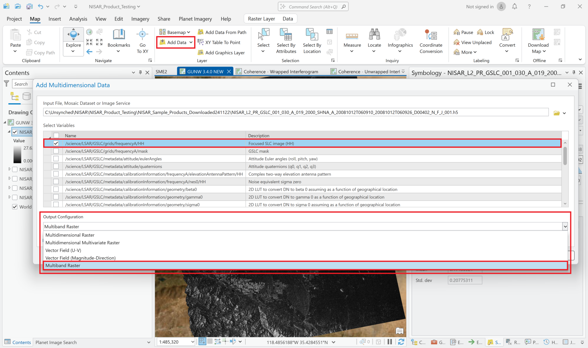
To extract the phase values, you will need to add the SLC variables as Multiband Rasters, so we’ll start with that method, then go over the rest of the options.
Add Multiband Rasters
In the Map tab, click the down arrow next to the Add Data button and select Add Multidimensional Data. Navigate to the GSLC HDF5 file, and select it to open the list of variables. Select the focused SLC variable. Click the drop-down menu under Output Configuration and select Multiband Raster, then click OK to add the variable.
Note that the sample data only includes one polarization for the SLC products, but actual NISAR data will often have multiple polarizations available.
By default, ArcGIS Pro displays the Amplitude values when a complex raster is added to the map.
Drag and Drop
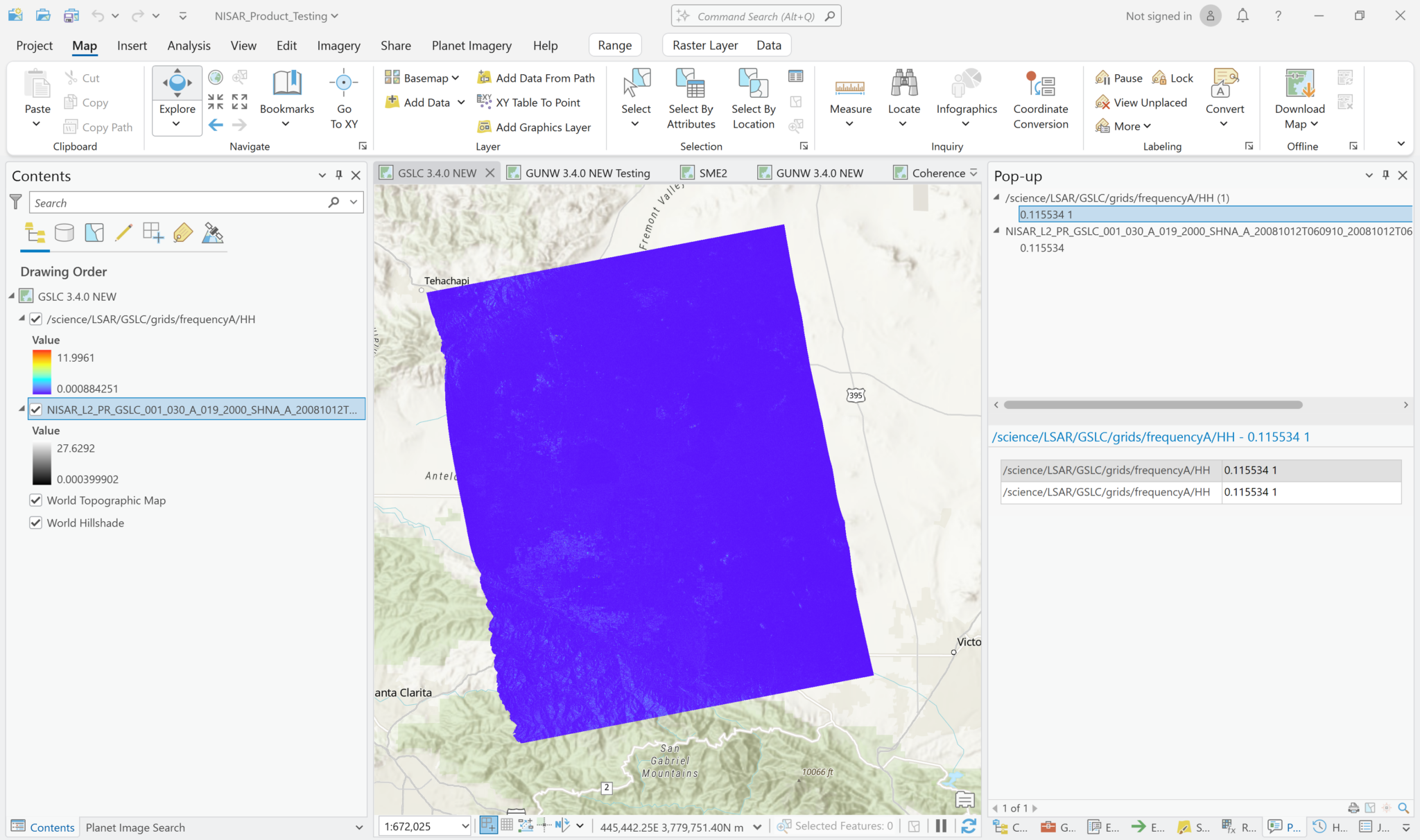
If you drag and drop the GSLC HDF5 file from the Catalog pane into a Map in ArcGIS Pro, the first variable in the HDF5 file is displayed. The sample GSLC files only have two gridded frequency variables, and the first is the focused SLC image in HH polarization. The values in the SLC variables are in 64-bit complex format, so if you do use the drag-and-drop method, you will only be able to access the Amplitude measurements (which are displayed by default).
Note that the software will try to calculate the statistics for the dataset, and it will keep trying for a very long time. You can cancel this effort to view the image with estimated statistics.
Because the statistics were not calculated, the range of values in the legend will likely be different from the layer added as a Multiband raster. If you click on a pixel, however, both layers return the same pixel value.
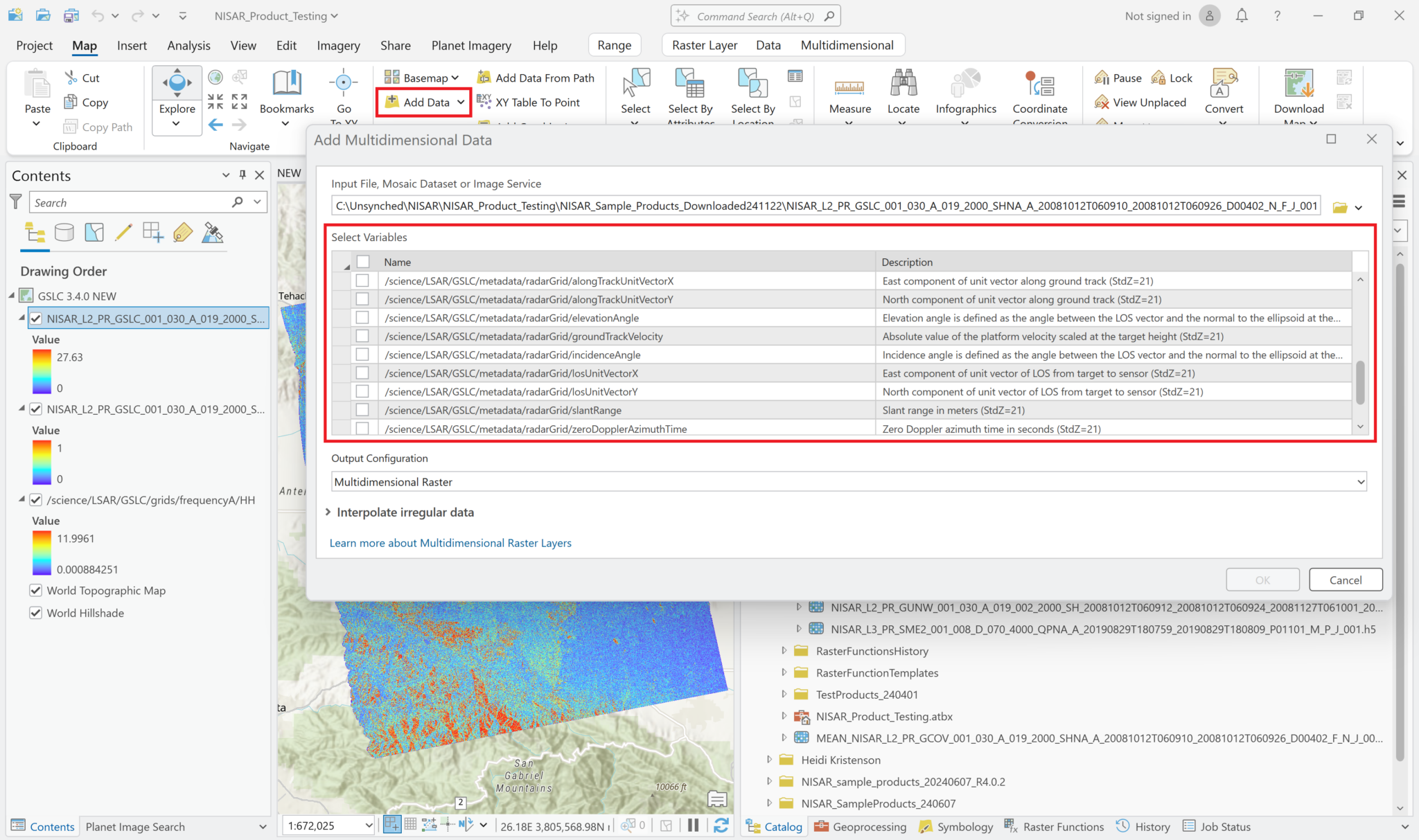
Add Multidimensional Data – Individual Variables
You can also add variables from the GSLC files as multidimensional rasters. Again, you will only be able to access the amplitude measurements in the SLC variables, but there are other variables that are better suited to this approach.
The other gridded frequency variable is the validity mask, but the variables in the /metadata/radarGrid path can also be visualized in ArcGIS Pro. These variables include along-track unit vectors, elevation angles, ground track velocity, incidence angles, LOS unit vectors, slant range, and Zero Doppler Azimuth time.
To add individual variables, click the drop-down arrow on the right side of the Add Data button, and select Add Multidimensional Data. Navigate to the GSLC HDF5 file and select it to view the available variables.
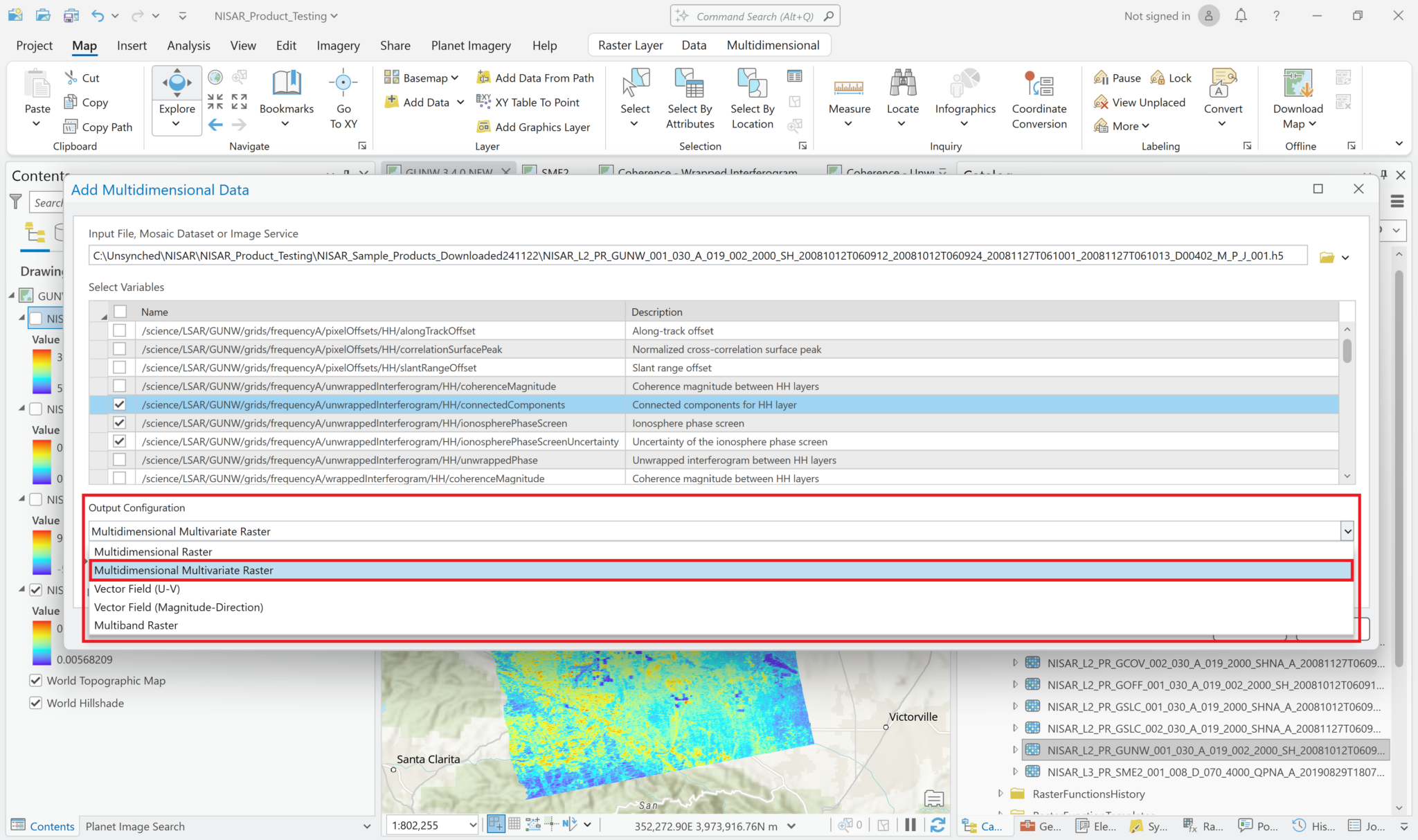
Click one or more of the variables listed, and leave the Output Configuration set to the default of Multidimensional Raster. Click the OK button to add the variable(s) to the map. If you select multiple variables, they will each be added as individual layers.
Add Multidimensional Data – Multivariate
It is also possible to add multiple variables to the project as a single layer. Use the same approach as when adding single variables to browse to the HDF5 file and view the list of variables to add. Select the desired variables, but instead of leaving the Output Configuration set to the default of Multidimensional Raster, use the drop-down Output Configuration menu to select Multidimensional Multivariate Raster.
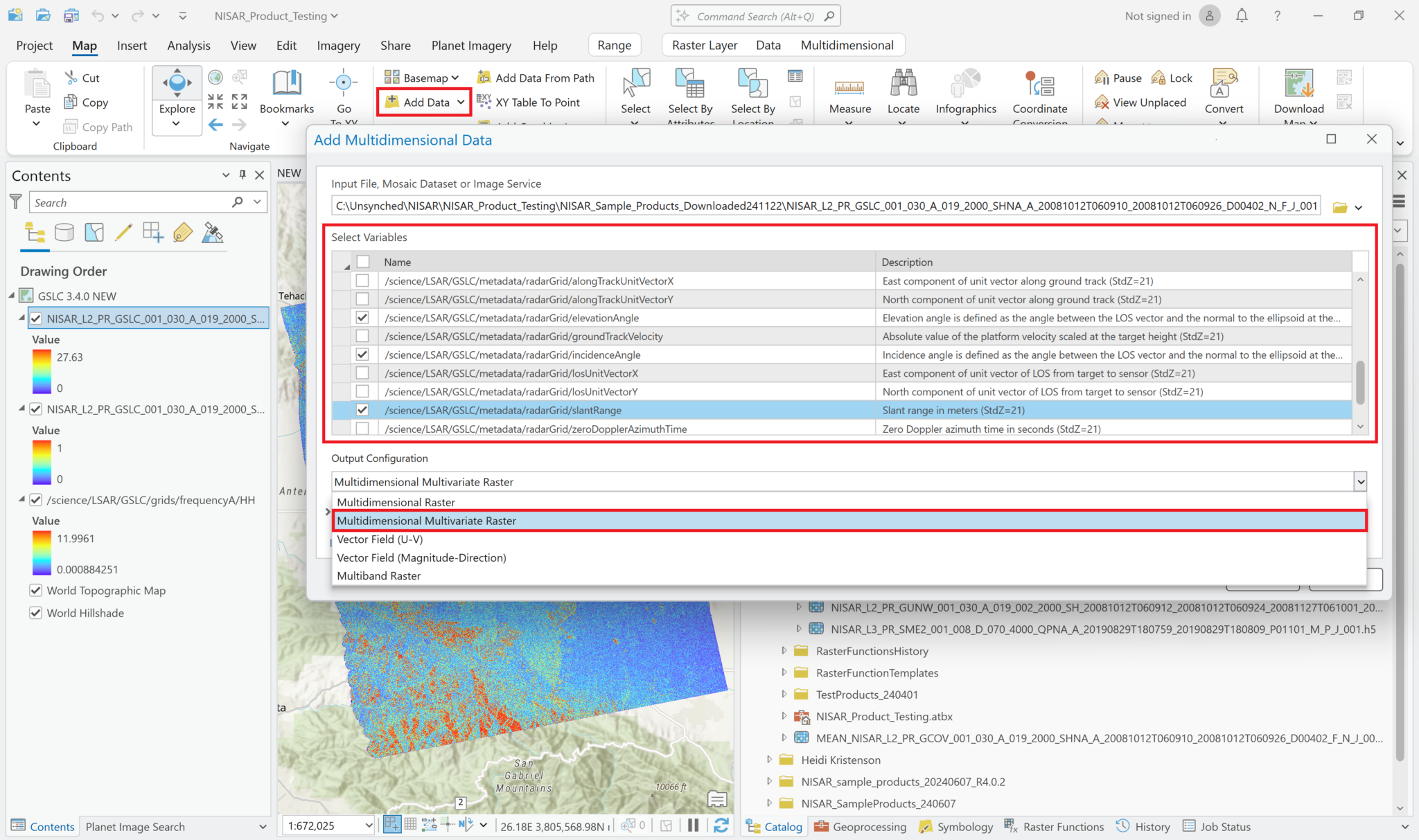
This adds a single layer to the map, labeled with the filename only (no variables indicated). The different variables that were selected can be accessed using the Multidimensional menu available when you click on the layer in the Contents pane.
Keep in mind that the same constraints apply to visualizing the complex-valued SLC variables; you will only be able to view the amplitude values.
Visualizing GSLC Products
The focused SLC variables in the GSLC products have complex pixel values, which include both real and imaginary components. ArcGIS Pro offers a Raster Function that allows you to extract either the Amplitude or the Phase measurements from the complex numbers, but the variables must be added using the Multiband Raster output configuration in order to use this functionality. You can then adjust the visualization of the output raster as desired.
Any of the other variables in the GSLC product (the validity mask or any of the variables in the radarGrid path) can be visualized as you would any other raster.
Apply Complex Raster Function
Click on the Raster Functions button under the Imagery menu to open the Raster Functions window. Either type Complex into the search bar, or expand the SAR menu and click the Complex button.
This opens the dialog window for the Complex raster function. Select the same layer (focused SLC variable) for both the real and imaginary inputs. The layer must have been added as a Multiband Raster.
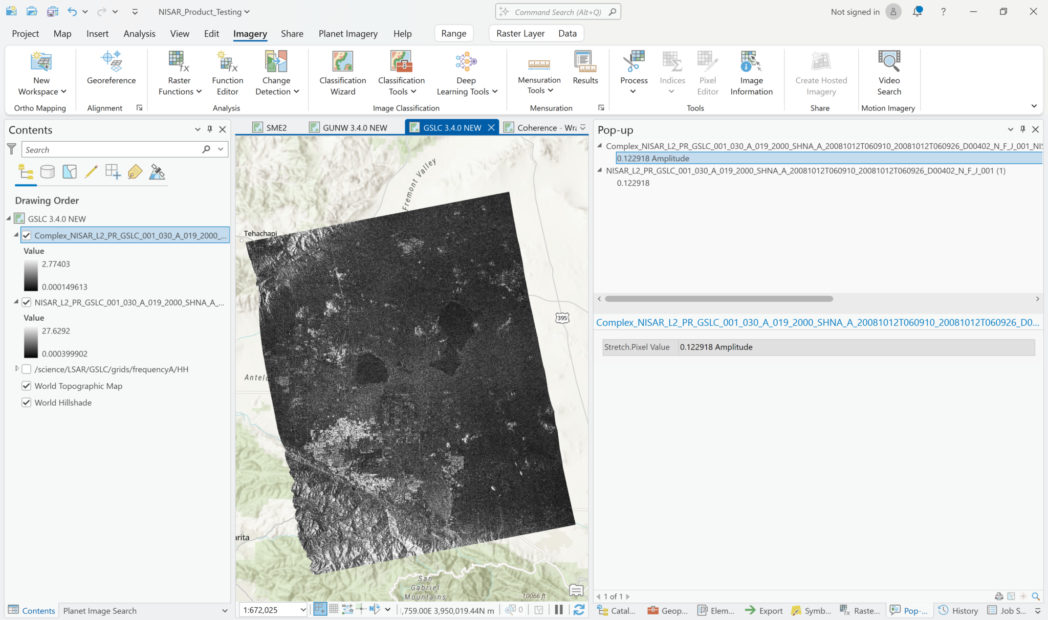
For the value type, select either Amplitude or Phase, then click the button to Create new layer. This will add a virtual layer to your map project. Alternatively, select Save As from the drop-down menu instead of Create new layer if you want to save the amplitude or phase output a new file for use in other projects.
If you select Amplitude, the output product will have the same values as the default visualization of the product. Again, the range of values in the legend may be different due to the calculation/estimation of statistics, but if you click on pixels, the values will be the same.
If you select Phase, the output product will have values ranging from -3.14 to 3.14. Generally the phase is not very informative visually, with what looks like a random pattern.
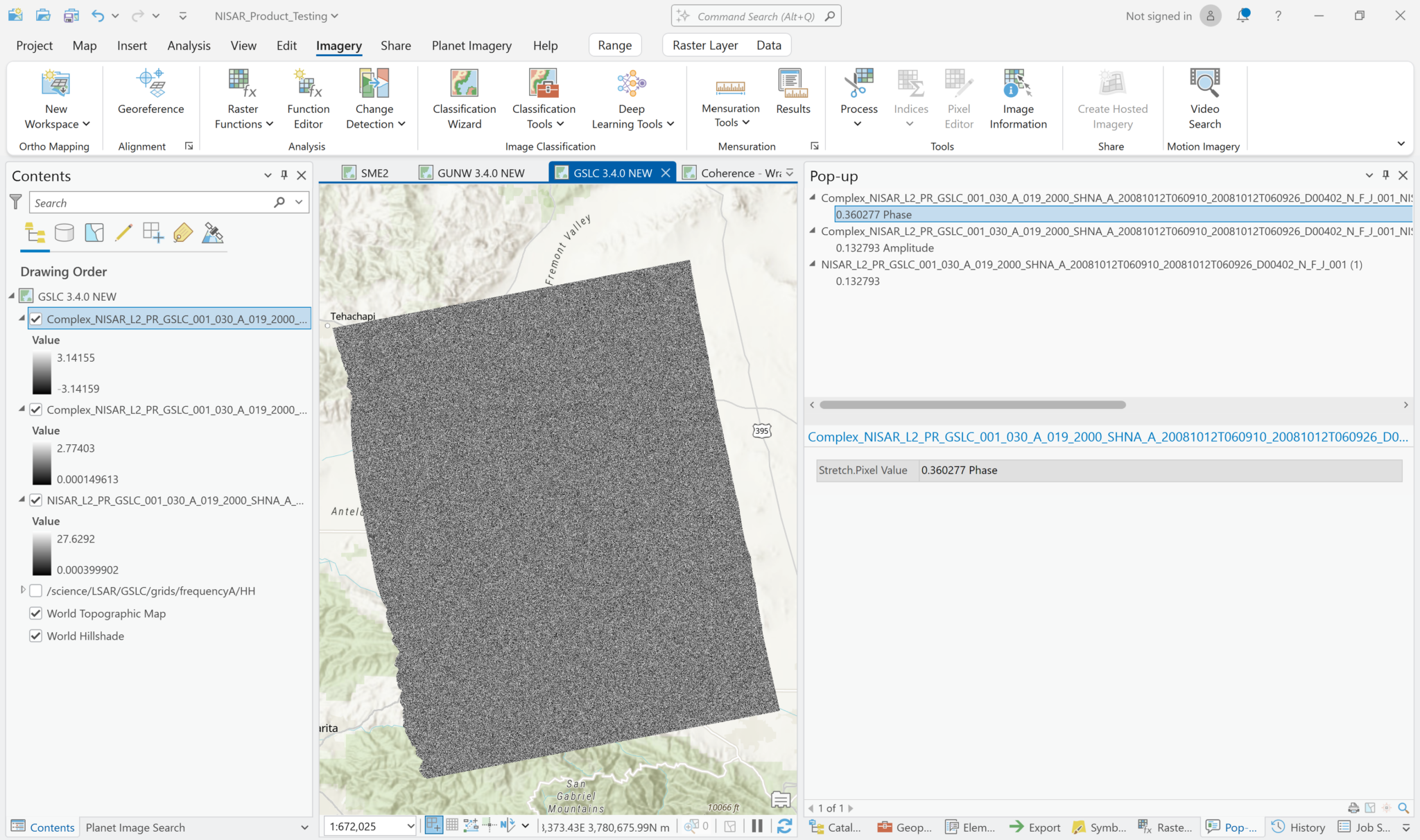
Note that the output layer is labeled with a Complex prefix in the Contents pane, regardless of whether you selected Amplitude or Phase. You may want to edit the layer name if you want to add both to your map.
When you click on a pixel, however, the value displayed in the pop-up window includes an indication of whether you’re looking at amplitude or phase, even though the layer names are the same.
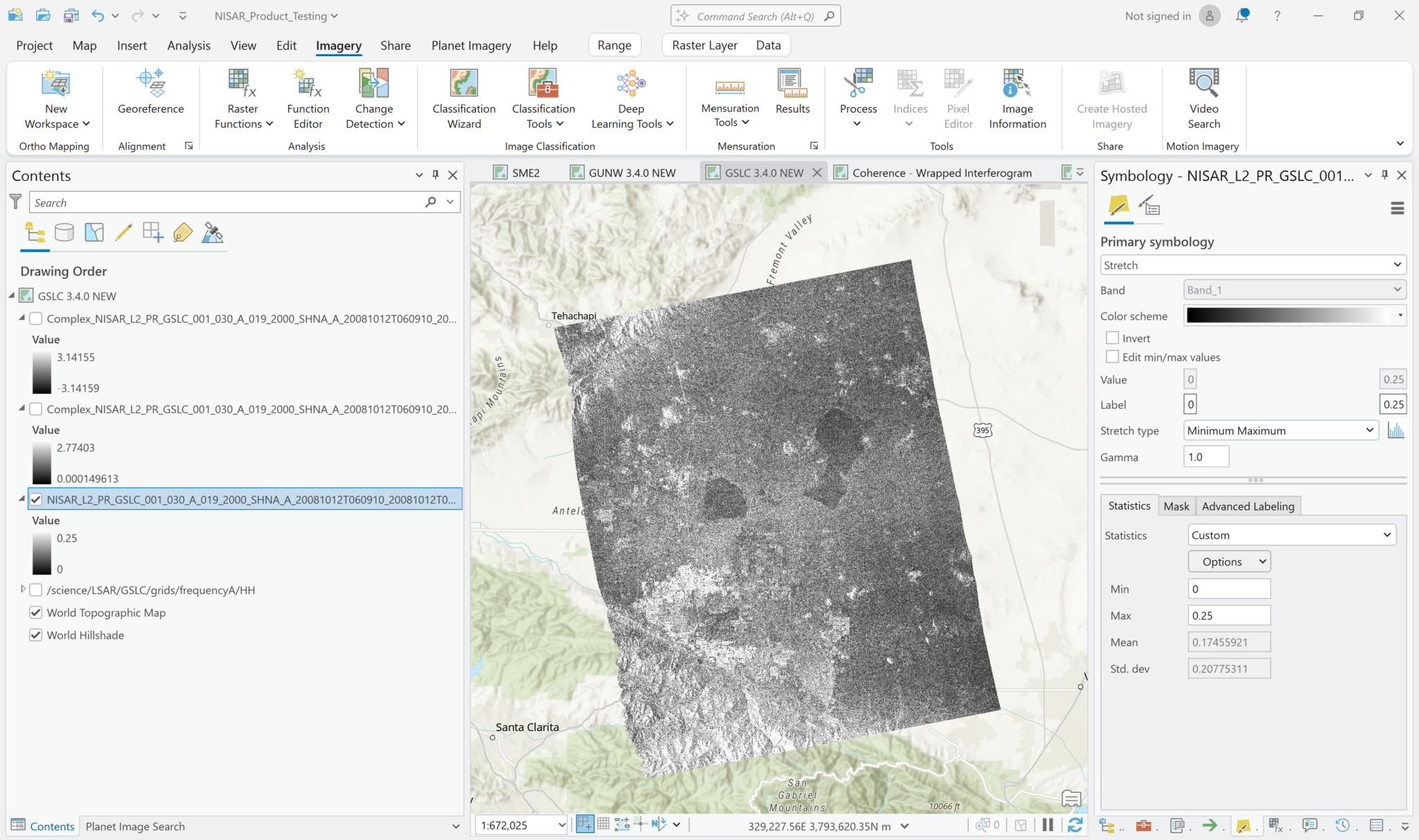
Symbology for Amplitude Measurements
You can use the same visualization approaches as with the GCOV products when viewing the samplitude component of the dataset. Right-click the layer in the Contents pane, and select Symbology. You can adjust the color scheme, the stretch type, and the range of values used for the stretch.
Because the amplitude values aren’t calibrated backscatter, the value ranges that work well may be different from what you would use with the GCOV products. For example, here is the GSLC amplitude image with a Minimum-Maximum value range set to 0 and 0.25. The visualization has much different contrast characteristics than what those same settings rendered for the GCOV product.
Symbology for Phase Measurements
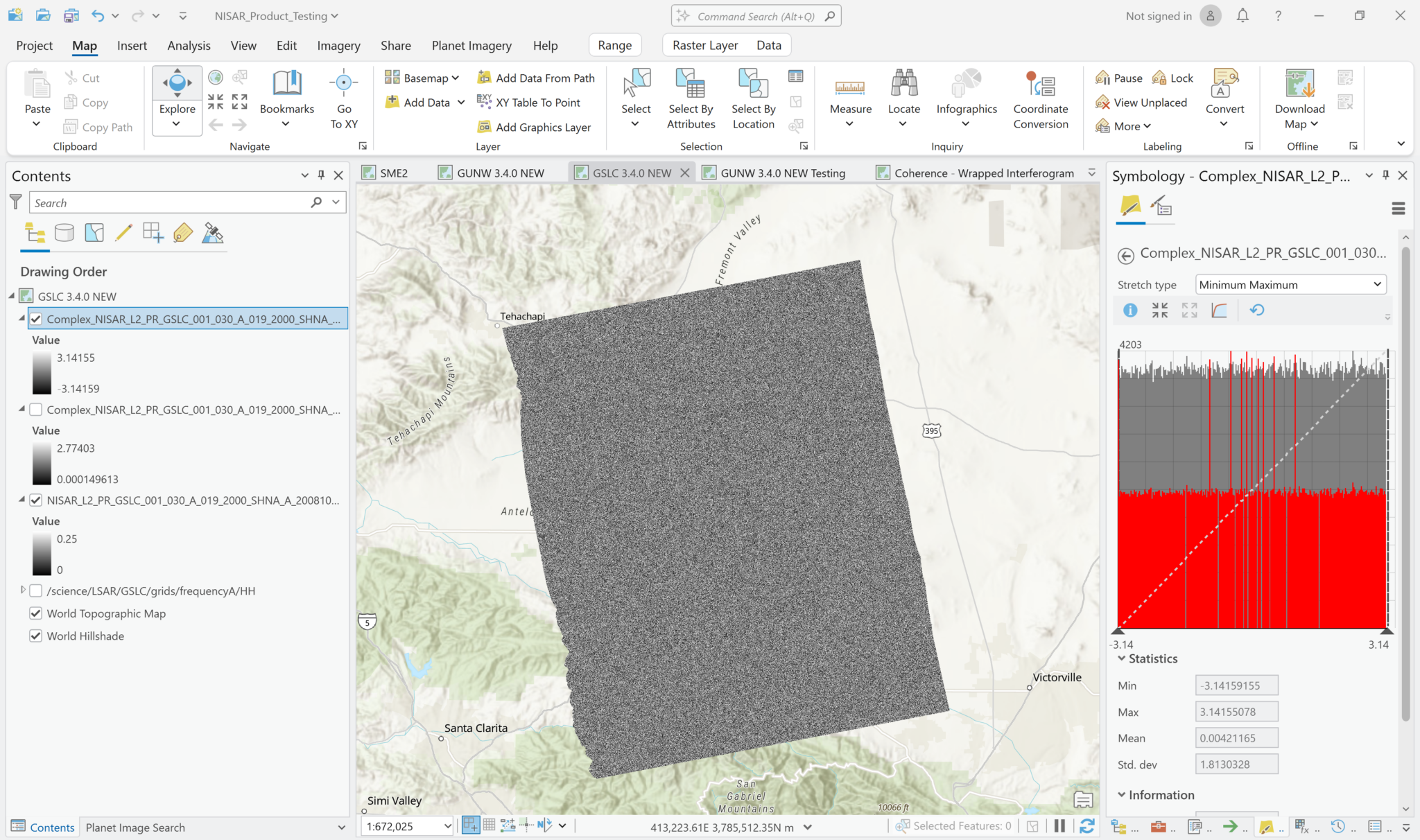
There’s generally not much to explore visually with GSLC phase measurements. If you click the Histogram icon next to the Stretch type in the Symbology pane, you can see that the pixel values are fairly evenly distributed across all values. As such, it doesn’t make much difference visually if you apply a Minimum-Maximum, Percent Clip, Standard Deviation, or Histogram Equalize stretch type.
There are two sample GCOV products available, one for each of the acquisitions used in other sample products that require imagery pairs:
NISAR_L2_PR_GCOV_001_030_A_019_2000_SHNA_A_20081012T060910_20081012T060926_D00402_N_F_J_001.h5
NISAR_L2_PR_GCOV_002_030_A_019_2000_SHNA_A_20081127T060959_20081127T061015_D00402_N_F_J_001.h5
The illustrations displayed in this document use the acquisition from November 27, 2008.
HDF5 Format
All NISAR products will be in HDF5 format, but they are formatted in such a way that most software applications need to treat them as if they are netCDF files.
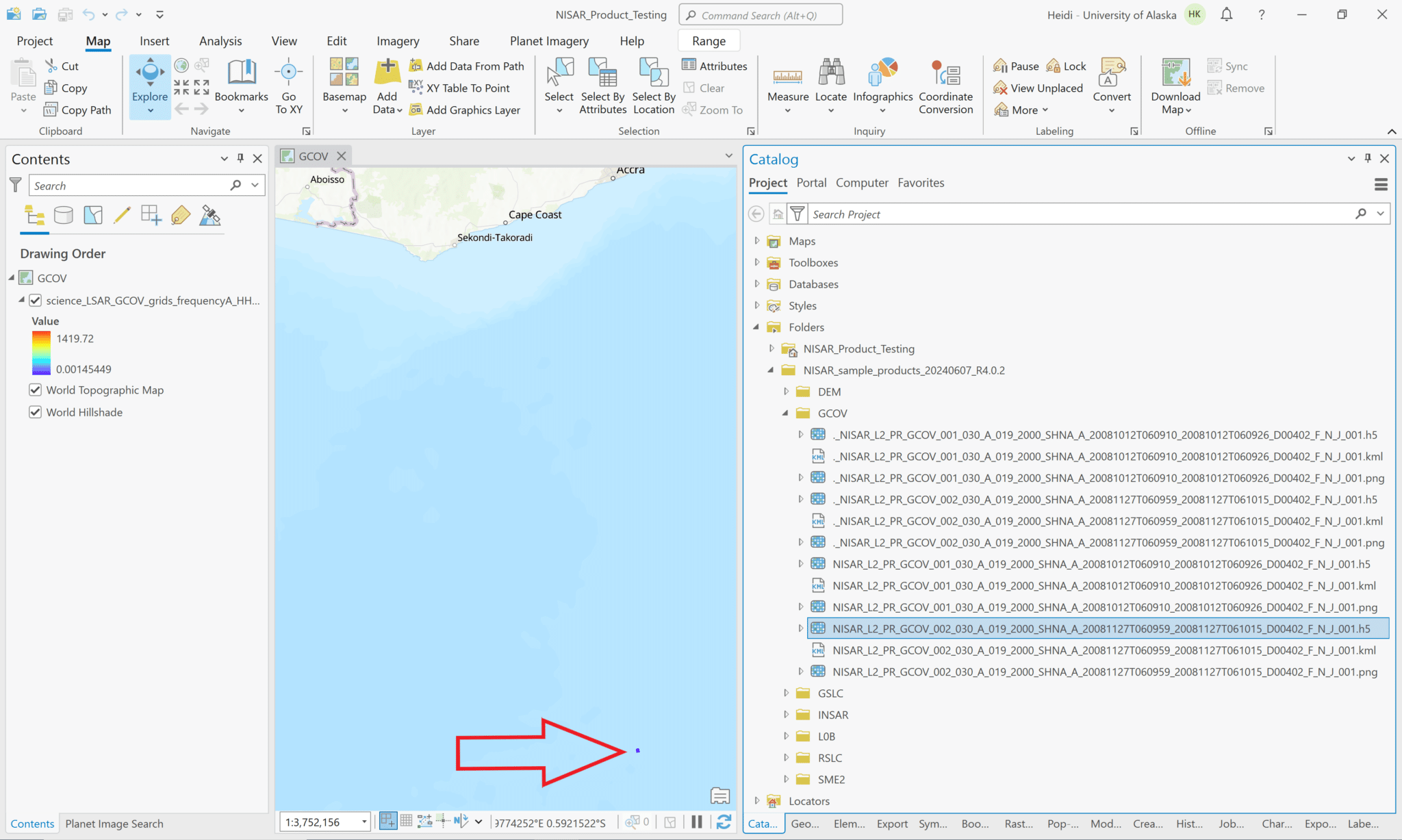
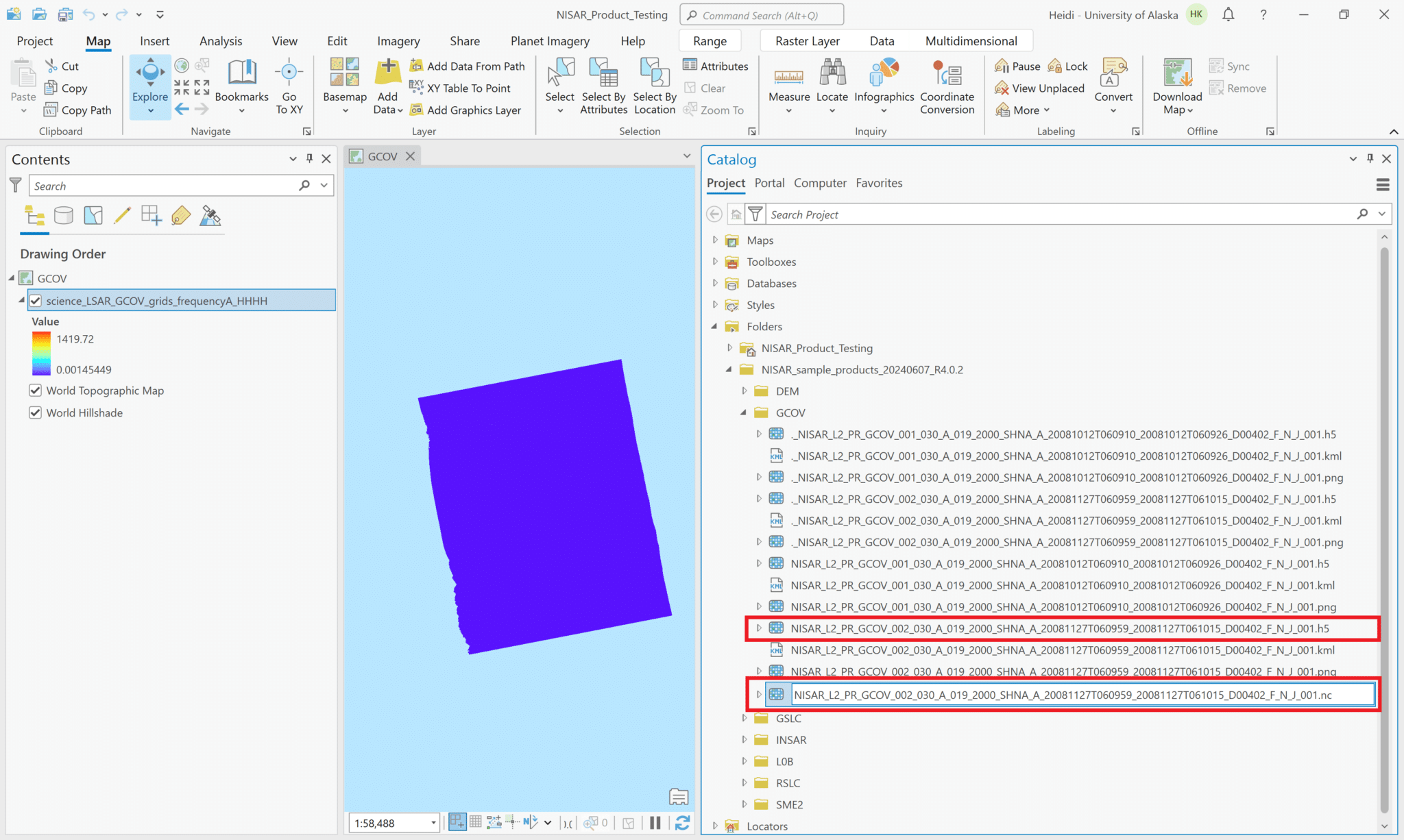
First, let’s explore what happens if we try to add the h5 file to the project.
- Navigate to the directory with the sample data files in the Catalog pane
- Note that the .h5 files are listed in the Catalog pane and are available to drag and drop into the project.
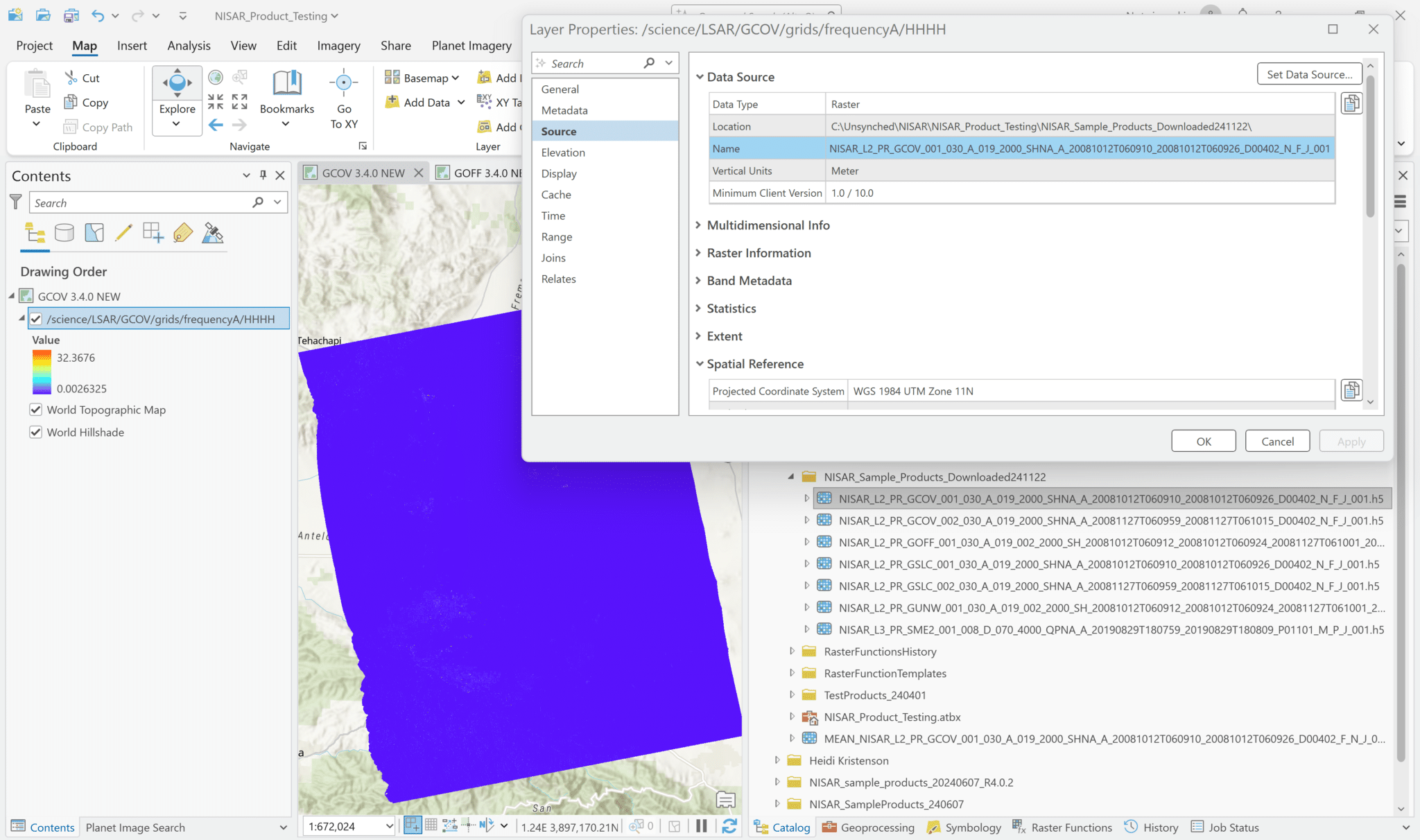
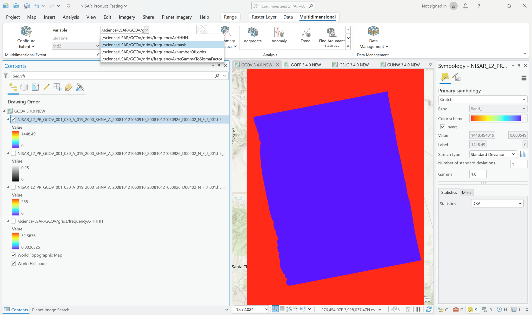
- When you add the HDF5 file to your map, it displays the L-band HH GCOV data in the map, but ArcGIS cannot access the spatial reference information and places the raster off the west coast of Africa. In the illustration below, the raster shows up as a small purple rectangle in the ocean.
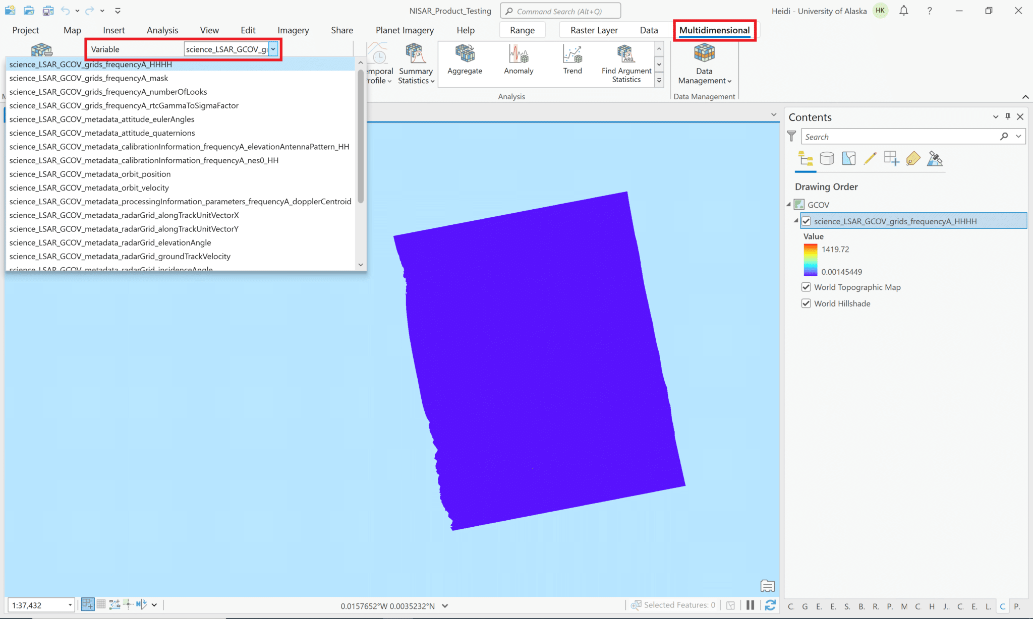
If you add the entire HDF5 file to the project, either by using the drag-and-drop method or by clicking the Add Data button and selecting the HDF5 file, you can access all of the variables in the dataset using the Multidimensional menu. Note that the Multidimensional menu only appears once you add a multidimensional dataset to your project and select it in the Contents pane.
By default, the first variable in the dataset will display in the map, but you can choose to display any of the other variables by selecting it from the drop-down list. The name displayed in the Contents pane will not change, but the map does display the data of the selected variable. You can adjust the symbology as appropriate for the variable you have selected.
Note that only the variables in the grids group will reliably display on the map. Many of the variables in the metadata group are not suitable for visualization.
- To view the raster properties, either right-click the file in the Catalog pane or right-click the layer in the Contents pane and select
Properties. It’s easier to see the key properties in a unified view when accessing the properties from the Catalog pane rather than the Contents pane.
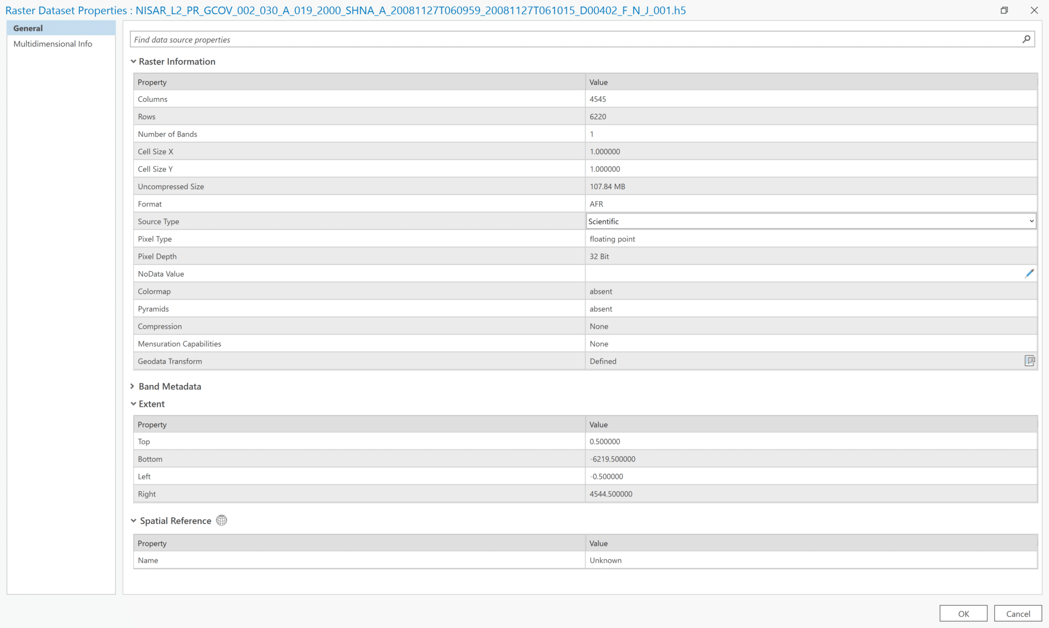
- Note that the Spatial Reference is listed as
Unknown
There is no metadata formatted in a way that can be accessed using the View Metadata option (right-click the file in Catalog pane), so the only insight into the dataset is what is displayed in the fields included in the dataset properties.
Treat HDF5 as NetCDF
The spatial reference information is encoded in the product using the CF metadata conventions, which were developed for use with NetCDF files. As such, if the GIS software recognizes the file as being a NetCDF, it can parse the spatial reference information and place the raster in the correct location. The current workaround for working with the NISAR HDF5 files in geospatial workflows is to rename the file with a .nc extension in place of the .h5 extension.
Change the file extension
- Browse to the HDF5 file in either a file explorer window or in the Catalog pane of your ArcGIS project.
- Edit the filename, changing the
.h5extension to.nc.- Note that once the extension has been changed, the file is no longer visible in the Catalog pane in ArcGIS. You can still add the file using the Add Data interface, but there will be no indication in the Catalog pane that this file exists.
- You can also copy and paste the .h5 file, and rename the copied file with the .nc extension. This can serve as a reminder that the data exists, but it takes up more storage space.
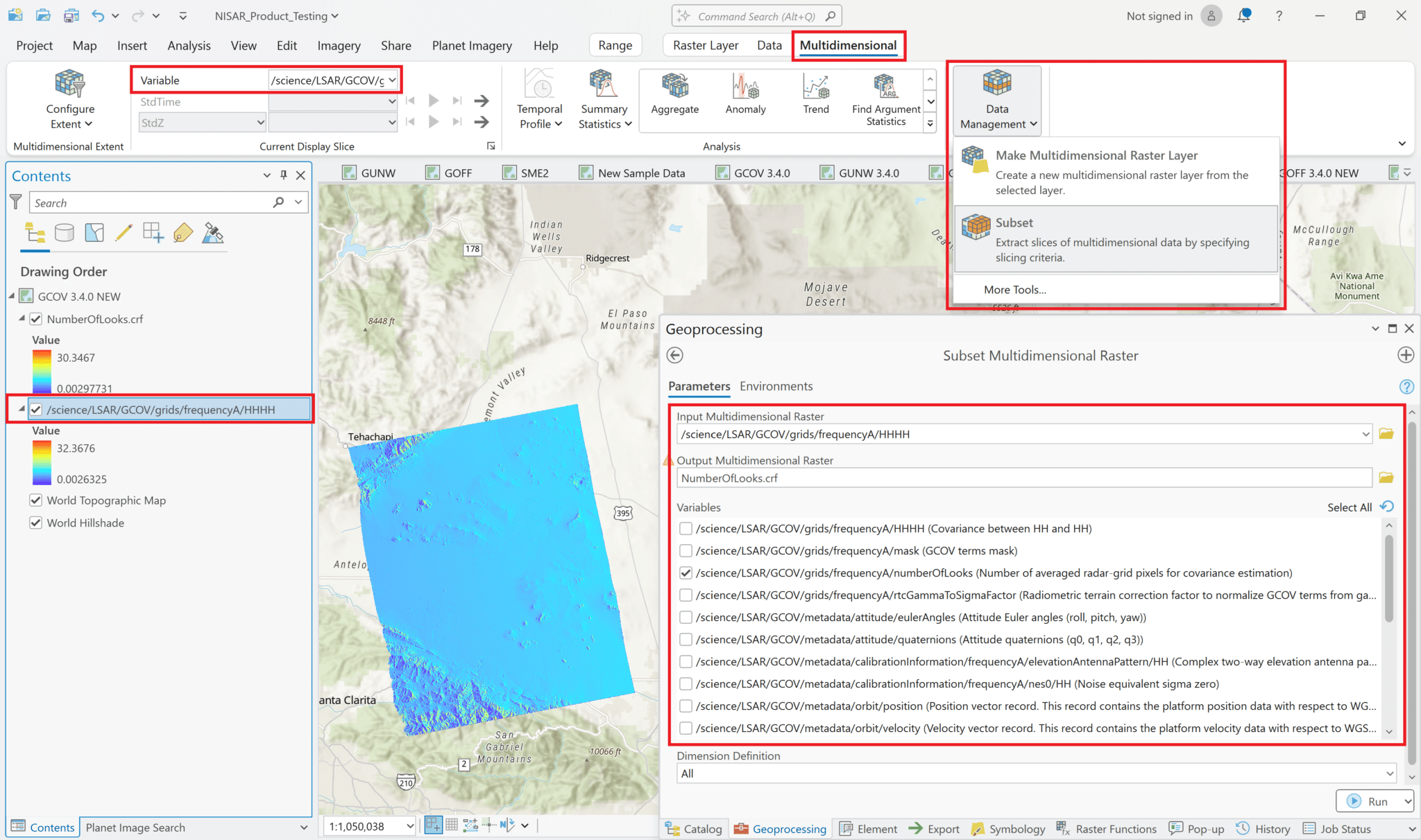
Add Single Variable from Multidimensional Raster to Project
- Click on the bottom half of the Add Data icon in the Map menu ribbon to display the menu, and select
Multidimensional Raster Layerfrom the list of options.- Note that if you just use the generic
Add Dataoption, you will be able to navigate to the .nc file, but there will be an error if you try to add it to the map, as it requires the functionality of theMultidimensional Raster Layeroption to access the variables within the .nc file.
- Note that if you just use the generic
- Click on the folder icon and browse for the NetCDF version of the HDF5 file.
- Note that HDF5 files are indicated by a blue raster icon, while NetCDF files are indicated by a multilayer grayscale raster icon.
- Select the NetCDF file and click OK. The variables in the HDF5 file will be listed.
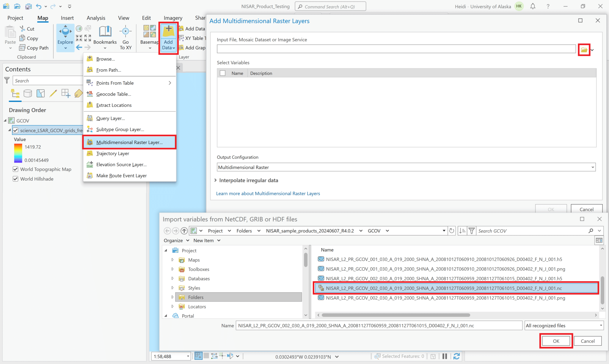
- Check the box next to the radar backscatter variable to add it to the project. In this sample product, only one polarization is available.
- Use the drop-down menu for the Output Configuration parameter to select
Multiband Raster.- It is critical to select this option; ArcGIS will not render the data if any of the multidimensional options are selected for the Output Configuration.
- It is possible to select multiple variables to combine into a single multiband raster, if desired. For most geospatial analysis applications, this is probably less convenient than adding the variables separately, but it is a convenient way to add many variables to the map at once for a quick exploration. Refer to the Add Multiple Variables from Multidimensional Raster to Project section for more details.
- Click OK to load the variable into the map.
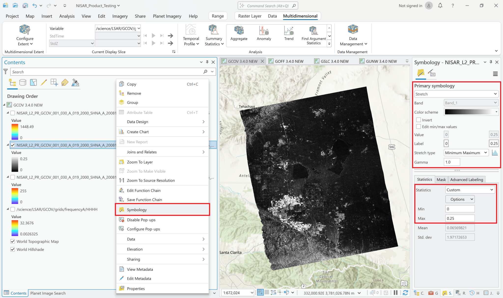
Adjust Stretch
As with most SAR backscatter images in power scale, the image appears mostly black when it’s added to the map. You can adjust the stretch settings to view features in the image.
- Right-click on the layer in the Contents pane and select Symbology

- Adjust the settings to visualize the layer as desired. Common approaches include:
- Set the Stretch Type to
Standard Deviationand adjust the Number of standard deviations value as desired. – For this sample image, 0.5 seems to be a reasonable value. – Changing the Gamma value from 1 to 2 reduces the amount of contrast in the mid-level grayscale values, adding more nuance to the image.
- Set the Stretch Type to
Minimum Maximumand selectCustomfrom the Statistics drop-down menu. This allows you to set a specific range of values to use for the grayscale in the Min and Max fields. Use the tab button after entering each value so that the label field is updated appropriately.- Normally, we would expect power values for RTC products to fall mostly between about 0 and 0.03, so we’ll use those for the Minimum and Maximum values.
- Again, adjusting the Gamma setting changes the character of the visualization.
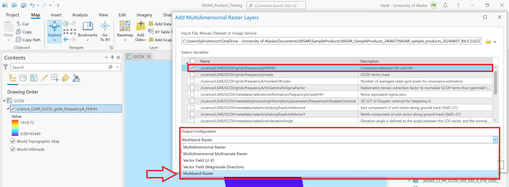
Add Multiple Variables from Multidimensional Raster to Project
This option could be particularly useful when there are multiple polarizations that you want to visualize quickly, especially if you want to use the different polarizations in different channels to display an RGB Decomposition.
- Follow the same steps as in Add Single Variable from Multidimensional Raster to Project to select the NetCDF and list the variables.
- Check the boxes next to the variables you want to include.
- Only the variables in the
/grids/group in the HDF5 file are suitable to use when adding multiband rasters with multiple variables.
- Only the variables in the
- Select the Multiband Raster from the Output Configuration drop-down menu, and click OK to add the multiband raster to the image.
Adjust the symbology to visualize the different bands as desired. By default, if three different variables are included, the image will be visualized as an RGB image with each of the variables assigned to a different band. If fewer than three variables are included, the image will be a grayscale stretch, and you can select which variable to display from the Symbology menu.
It is critical to allow the imagery to render fully each time you change a symbology setting before adjusting another symbology setting.
For example, if you change to a Standard Deviation stretch, allow the image to render fully before changing the number of standard deviations.
Here are some notes on visualization options:
- In some cases, it may make sense to keep the RGB visualization. This could be particularly powerful if you’re interested in combining the variables to display particular properties. The best use case is probably for images with multiple polarizations, but because the sample data only includes HH, there are no other polarizations available to be used in combination with HH to generate an RGB decomposition.
- In this illustration, three variables available in the grid group are assigned to the RGB channels. Because the backscatter values are so small compared to the range of values in the other two variables, there is essentially no red in the image.
- You can adjust the stretch type within the RGB image to highlight particular values/features. However, the variables available for use in this example do not offer a particularly compelling use case for this functionality.
- In this illustration, changing the stretch type to Standard Deviation allows you to see areas with high backscatter in relation to the other two variables.
- Setting the number of standard deviations to 0.5 would make the range of backscatter values even more obvious.
- When two variables are added (rather than three), the image displays as grayscale stretch by default, and you have to choose which variable to display. You can, however, change the symbology from Stretch to RGB and assign one of the variables to two of the color bands.
- This would be particularly useful for dual-pol imagery, where a common approach for is to apply the co-pol (usually HH for NISAR) data to the Red and Blue channels, and the cross-pol (usually HV for NISAR) data to the Green channel.
The illustrations in this section display the previous version of the sample data, and use ArcGIS Pro version 3.2.2 rather than 3.3.0. The workflow is the same with the new products, and there are only minor changes in the ArcGIS interface.
The sample GUNW data file is:
NISAR_L2_PR_GUNW_001_030_A_019_002_2000_SH_20081012T060912_20081012T060924_20081127T061001_20081127T061013_D00402_M_P_J_001.h5
Note that most of the variables in this file have float or integer pixel types, but the wrapped phase variable has a complex pixel type. ArcGIS can display all of the variables, but refer to the Wrapped Phase section for details on how to appropriately visualize complex datasets. This table describes the pixel types for all of the variables included in the grids group of the h5 file:
| Variable | Pixel Type |
|---|---|
| /science/LSAR/GUNW/grids/frequencyA/pixelOffsets/HH/alongTrackOffset | 32-bit float |
| /science/LSAR/GUNW/grids/frequencyA/pixelOffsets/HH/correlationSurfacePeak | 32-bit float |
| /science/LSAR/GUNW/grids/frequencyA/pixelOffsets/HH/slantRangeOffset | 32-bit float |
| /science/LSAR/GUNW/grids/frequencyA/unwrappedInterferogram/HH/coherenceMagnitude | 32-bit float |
| /science/LSAR/GUNW/grids/frequencyA/unwrappedInterferogram/HH/connectedComponents | 32-bit unsigned integer |
| /science/LSAR/GUNW/grids/frequencyA/unwrappedInterferogram/HH/ionospherePhaseScreen | 32-bit float |
| /science/LSAR/GUNW/grids/frequencyA/unwrappedInterferogram/HH/ionospherePhaseScreenUncertainty | 32-bit float |
| /science/LSAR/GUNW/grids/frequencyA/unwrappedInterferogram/HH/unwrappedPhase | 32-bit float |
| /science/LSAR/GUNW/grids/frequencyA/unwrappedInterferogram/mask | 8-bit char |
| /science/LSAR/GUNW/grids/frequencyA/wrappedInterferogram/HH/coherenceMagnitude | 32-bit float |
| /science/LSAR/GUNW/grids/frequencyA/wrappedInterferogram/HH/wrappedInterferogram | 64-bit complex |
Data from this file can be accessed using the same workflow described for the GCOV Product.
- Change the file extension from .h5 to .nc
- Use the Multidimensional Raster Layer option in the Add Data menu to browse to the .nc product and select the variables to add to the map.

The most common variables to visualize are the wrapped and unwrapped interferograms and the coherence magnitude, but any of the variables in the \grids\ subgroup are rasters that can be displayed in a GIS environment.

As with the GCOV products, the output configuration selected when adding variables must be Multiband Raster, but you can choose to add individual variables as separate rasters (technically a single-band raster, but still defined as a multiband raster), or select multiple variables to be added to the map together in a single multiband raster (that truly includes multiple bands, each with a different variable).
In general, if you’re interested in optimizing the visualization of a raster, it’s better to add the variable of interest by itself, rather than as a multiband raster that includes other variables. The more you tweak the symbology, the more likely you are to lose the connection to the file, and have to start over. If there’s only one variable included in the multiband raster, it seems to be more robust to symbology adjustments. That said, the connection to the source data can be lost even with a single-variable raster, especially if a symbology adjustment is made that calls for statistics.
When you first add a raster to the map, the variable names usually show up in the list of bands in the Symbology tab. This is the case both for rasters with multiple variables included, and those with just a single variable displayed in the raster, both for greyscale and RGB. This is an easy way to determine which variable you’re exploring.
Sometimes the band name gets lost, however, especially after changes are made to the symbology. Instead of the variable name being displayed in the Symbology tab, there is just the generic Band number listed. Because the name of the variable is not displayed in the contents pane by default, it is easy to lose track of which variable the raster represents. You may want to rename the raster layer in the Contents pane, or add an identifier to the end of the existing layer name.
In the illustration below, the wrapped interferogram variable name is no longer displayed in the Band field of the Symbology tab, so we can identify it by right-clicking the layer in the Contents pane, and selecting Properties. In the Source section, the Name field displays both the filename and the variable path.
Note that there is an option to Set Data Source in the properties. Normally, if you lose a connection to a dataset, you can use that option to select the source file and repair the connection. Unfortunately, because the .nc files are not recognized as ‘files’ by ArcGIS, this is not a viable option to use if you lose the connection to the file while adjusting the symbology. If you try to navigate to the folder with the .nc files, only the .h5 files are listed.
Wrapped Phase
The wrapped phase variable has a complex pixel type, containing both real and imaginary components that can be used to calculate either the amplitude or the phase. When looking at an interferogram to detect and quantify surface deformation, we’re interested in differences in phase rather than in amplitude. By default, however, ArcGIS displays the image in terms of the amplitude values instead of the phase, with pixel values ranging from 2.78641e-12 to 7.37396e-05 for the sample dataset.
Starting with version 3.0, ArcGIS Pro provides a ‘Complex’ raster function, which can be used to display the phase values instead of amplitude values. It is included in the SAR section of the raster functions panel in ArcGIS Pro.
- Add the wrapped interferogram variable to the map
- You may want to rename the layer to ‘wrapped interferogram’ if there are already multiple layers from the NetCDF file, as it will make it easier to select the appropriate layer in the raster function interface
- From the
Imagerymenu, selectRaster Functionsto open the Raster Functions panel - Type
Complexin the search bar at the top of the Raster Functional panel, and click on theComplexraster function - Select the wrapped interferogram layer in both the Raster and the Imaginary Raster fields
- Select
Phasefrom the Value Type drop-down menu - Click the
Create New Layerbutton to display a layer showing the Phase values instead of the Amplitude values
The values displayed in the image now range from -pi to pi, which is what we would expect for a wrapped interferogram.
Note that the phase layer is a virtual raster that is displayed on-the-fly in your project, but you can export the layer as a stand-alone raster if you would like to save it for future use in other applications.
Coherence
There are two different coherence magnitude variables included: unwrapped coherence magnitude and wrapped coherence magnitude. They have slight differences in their values, but it’s unclear why. There doesn’t appear to be any guidance on which one would be preferable to use for particular applications.
Both versions have values ranging from 0 to 1, as expected for coherence values, and are easily displayed in grayscale without having to adjust the scale. In this illustration, both images were set to have a Min-Max stretch from 0 to 1 so that they could be compared visually, but the actual dataset min-max values are also displayed next to the functional scalebar for each image.

Mask
There is a layover-shadow mask included as a variable. It uses various integers to represent certain conditions, but I have not been able to find a reference for what the values represent. It is most useful to display this layer with a Discrete symbology, which applies a different color for each pixel value. In the sample data, there are three different pixel values present: 0, 2 and 127.
0 appears to indicate that there are no quality flags, and 127 indicates the padding pixels around the valid data. The pixels with a value of 2 are generally in the mountains, but it’s unclear if it indicates layover, shadow, foreshortening, or a combination of multiple conditions.

Click on the color patch next to each value in the symbology pane to manually select colors for each individual value. It can be helpful to set the 0 values to be transparent when viewing the mask in relation to an interferogram raster.
The sample GOFF data file is:
NISAR_L2_PR_GOFF_001_030_A_019_002_2000_SH_20081012T060912_20081012T060924_20081127T061001_20081127T061013_D00402_M_P_J_001.h5
There are 21 variables included in the grid group, seven variables for each of three different layers, generated with different window sizes. They are all 32-bit float datasets.
Data from this file can be accessed using the same workflow described for the GCOV Product.
- Change the file extension from .h5 to .nc
- Use the Multidimensional Raster Layer option in the Add Data menu to browse to the .nc product and select the variables to add to the map.
You may find it helpful to apply a color ramp to the products, rather than the default grayscale. In the Symbology settings for the layer, click the Color scheme menu to select a ramp that has two different colors at the extremities with a neutral color in between.
The sample SME2 data file is:
NISAR_L3_PR_SME2_001_008_D_070_4000_QPNA_A_20190829T180759_20190829T180809_P01101_M_P_J_001.h5
There are three different variables containing soil moisture data: DSG (Disaggregated), TSR (Time Series Rates), and PMI (Physical Model Inversion).
Data from this file can be accessed using the same workflow described for the GCOV Product.
- Change the file extension from .h5 to .nc
- Use the Multidimensional Raster Layer option in the Add Data menu to browse to the .nc product and select the variables to add to the map.
One key difference with this product is that you can add the variables using the Multidimensional Output Configuration. The other types of products require setting this option to Multiband Raster, but the SME2 variables can be added using either of these output configurations.
Adding a variable as a multidimensional raster allows access to the Multidimensional menu in the ribbon, but only the added variable will be accessible to select when using those tools.
Even if you select multiple variables and add them using the Multidimensional configuration, they will each be added to the map individually. Again, if you select one of the layers in the Contents pane, you can access the Multidimensional menu, but will only be able to access the variable represented in the layer. The name of the variable is added to the layer name in the Contents pane, which is very helpful.
To select multiple variables and add them to the map as a single content item, use the Multidimensional Multivariate configuration option.
This adds all the variables you select as a single layer in the Contents pane. When you select the layer, the Multidiminsional menu becomes available, and you can select the variable you want to visualize using the drop-down menu.
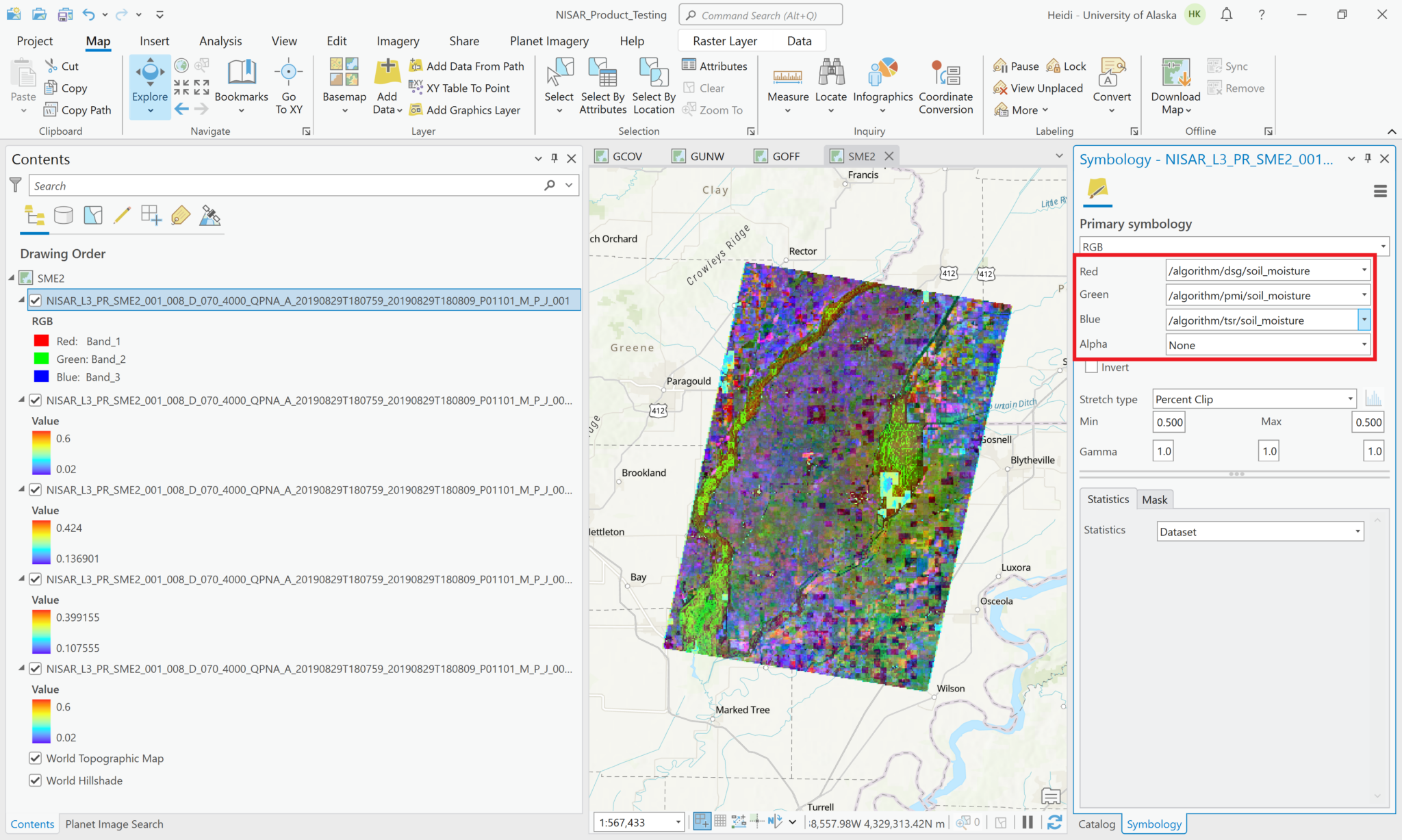
You can also use the Multiband Raster configuration to generate an RGB image from three variables.
In the Symbology tab, use the dropdown menus to select which variable to display for each color band.
In order to load the images into QGIS, you will have to replace the .h5 file extension with .nc. This is because the NISAR data is actually formatted like a NetCDF file, rather than HDF5. If you try to use the regular .h5 files, QGIS will likely crash (with no error or warning) when you choose a layer (refer to the QGIS Crashes section for more information). If you load the .h5 file, QGIS may continue to crash even after renaming to .nc. This may be fixed by deleting the .aux.xml file that QGIS creates in the same directory as the dataset.
Once you have the file named, you can simply drag and drop it into the QGIS window. This should bring up a prompt to select the desired layers. In our case, we want the layer that ends with HHHH.

You should now have something that looks like this:

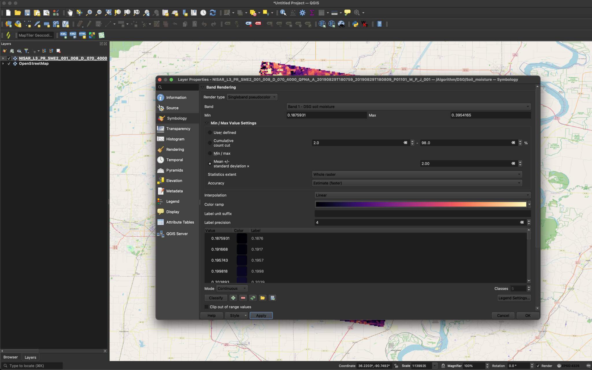
By default, QGIS scales the color map based off of the min and max. This leads to a dark image. We can fix this by changing the way that QGIS scales the color map. We can do this by right-clicking the layer and selecting Properties. We can then go to Symbology -> Min / Max Value Settings and select Cumulative Cut Count.

Now, things should look much better.

If you would like color, rather than a black-and-white image, you can click on the Render Type drop-down box in the Symbology page and select singleband psuedocolor. For this, you will also want to use Cumulative Cut Count.
Selecting the Desired Groups/Layers/Sub-Datasets?
Just like the GCOV products, we will first need to replace the .h5 extension with .nc, otherwise the projection information will be incorrect. Once the extension is replaced, we can drag the file into QGIS as normal and then select the desired layers. For this demonstration we will select the unwrappedInterferogram/HH/coherenceMagnitude and unwrappedInterferogram/HH/unwrappedPhase layers.

Unwrapped Phase
Now that the layers are added, we can right-click and zoom to the unwrapped phase layer. You should have something that looks like this:
While this image is relatively clear and interpretable, we can modify the symbology to bring out some more detail. We can do this by right-clicking the layer and selecting Properties. We can then go to Symbology -> Min / Max Value Settings and select Cumulative Cut Count or Mean +/- standard deviation.

When color is desired, you can also switch the Render Type to singleband psuedocolor in the same menu.
Coherence Magnitude
The coherence magnitude image should look good by default, but the same process that we applied to the unwrapped image can be applied if desired.

Wrapped Phase
Unlike the unwrapped phase and coherence magnitude, the wrapped phase data uses a complex data type. Unfortunately QGIS won’t natively handle complex data, so we will have to extract the phase component using this GDAL command:
gdal_translate -of GTiff DERIVED_SUBDATASET:PHASE:path/to/nisar.nc:/science/LSAR/GUNW/grids/frequencyA/wrappedInterferogram/HH/wrappedInterferogram phase.tif
We can then load the GeoTIFF image into QGIS as normal. It should look good by default, but you can modify the Symbology in the same manner as the unwrapped phase, if desired.

After changing the extension from .h5 to .nc, we can drag the file into QGIS and select the desired layers. Here, we will visualize the alongTrackOffset layer.
You can visualize the data without changing the symbology, but you can try varying the Min/Max Value Settings in the Symbology section of the layer properties if desired.
After changing the extension from .h5 to .nc, we can drag the file into QGIS and select the desired layers. Here, we will visualize the Soil_moisture layer.
The image should be easy to visually interpret by default.
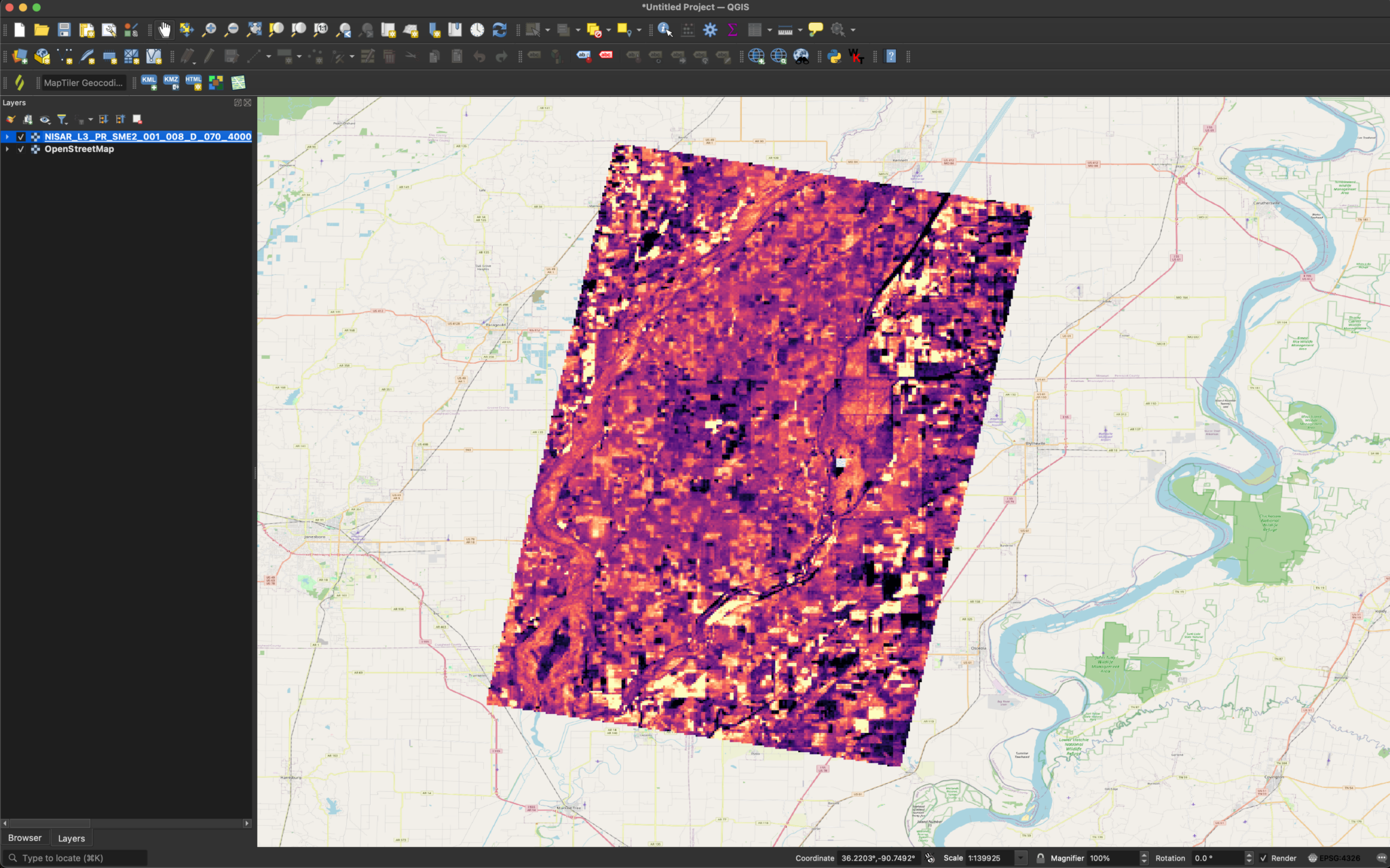
If desired, we can also add colored symbology and modify the Min/Max Value Settings. This will add more contrast, and can make things easier to interpret.
Once that is done, the image should look this:
QGIS does not have a way of natively viewing complex valued data, but we can use GDAL to extract the amplitude and phase components into separate real-valued images. Since the amplitude component contains the visual information, we will extract that using the following GDAL command:
gdal_translate -of GTiff DERIVED_SUBDATASET:AMPLITUDE:NETCDF:/path/to/nisar.nc:/science/LSAR/GSLC/grids/frequencyA/HH amplitude.tif
Note that we can also extract the phase component by replacing :AMPLITUDE: with :PHASE: if needed.
We can now load the image into QGIS.
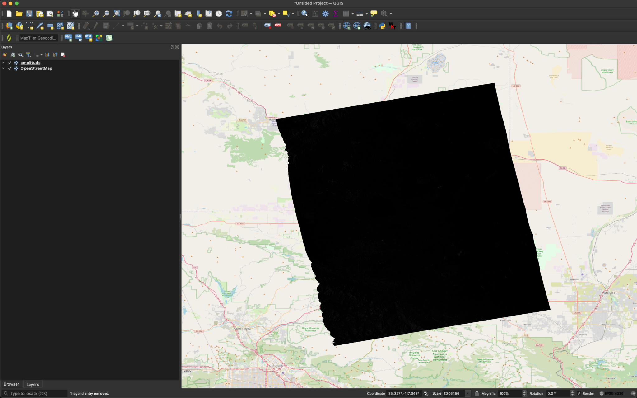
Without adjustments, the image will usually appear black. This is because QGIS defines the color range based on the maximum and minimum values, but SAR tends to have a small number of bright pixels that expand the dynamic range far beyond the majority of the pixel values. In order to visualize surface features, we can set the Min/Max Value Settings to Mean +/- standard deviation x in the Symbology section of the layer’s properties. This prevents the small number of very bright pixels from disproportionately affecting the grayscale range.
The image should then look like this:

The GUNW data file is
NISAR_L2_PR_GUNW_001_030_A_019_002_2000_SH_20081012T060912_20081012T060924_20081127T061001_20081127T061013_D00402_M_P_J_001.h5
1). Open the File
cd ${path_to_panoply}
./panoply.sh
The Panoply user interface opens as shown below.

- Navigate to the directory with the file in the Open window
- Click on the NISAR_L2_PR_GUNW_001_030_A_019_002_2000_SH_20081012T060912_20081012T060924_20081127T061001_20081127T061013_D00402_M_P_J_001.h5 file
- Click the
Openbutton to load the file into Panoply, as shown below
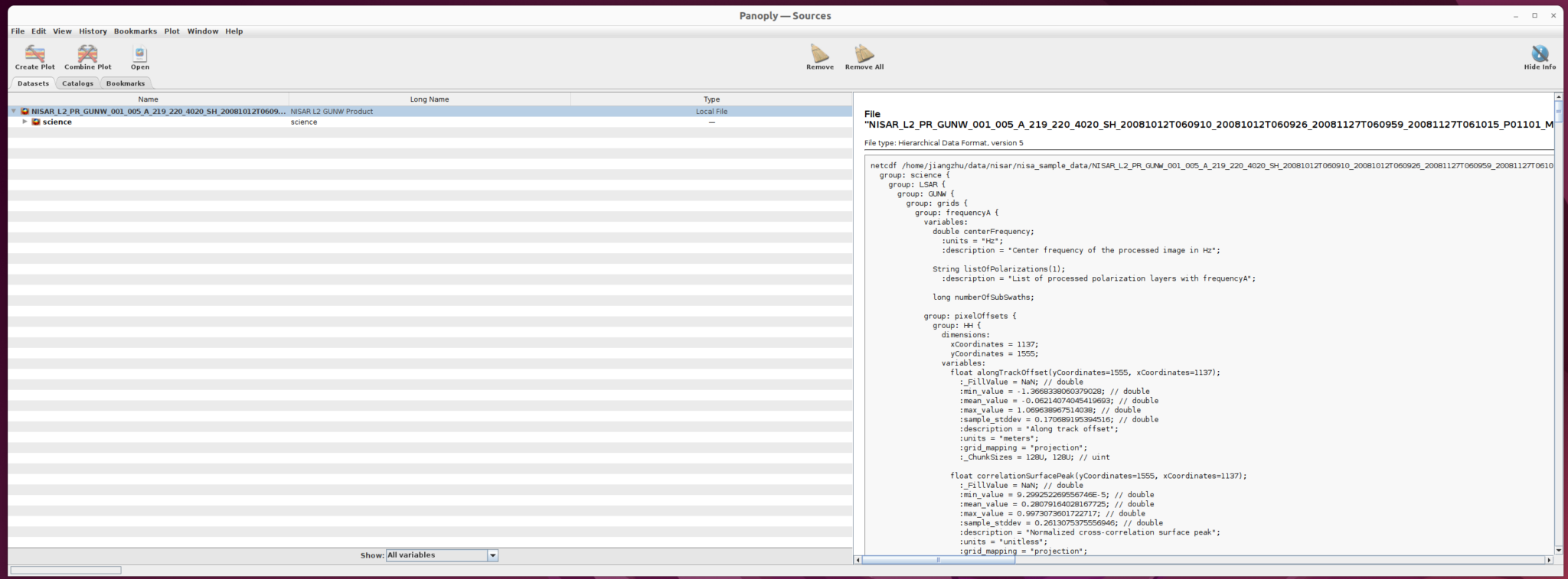
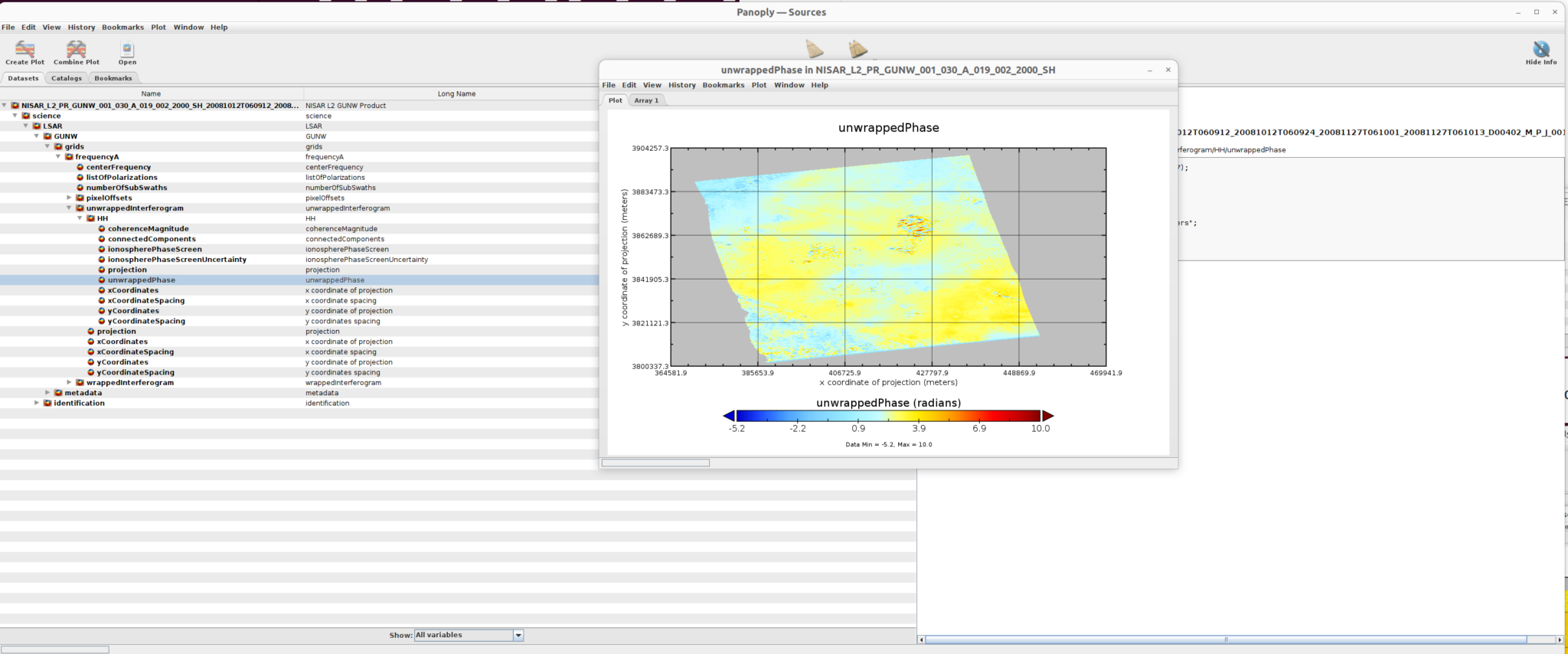
The right panel shows the structure of the file as well as the metadata. You can use this interface to inspect file information. The left panel provides users the option to select the dataset they want to use.
Expand the drop-down menu to find the “unwrappedPhase” dataset, which we will visualize in the following steps.

2) Create Plot
Once you select the dataset to use (in this case, unwrappedPhase), click the Create Plot button right below the main menu. A dialogue window opens with options for the type of plot to create.
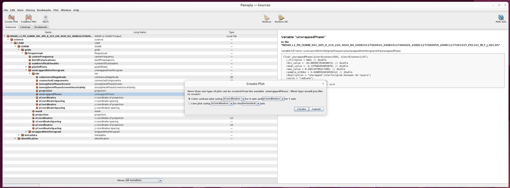
Select Color contour plot, then click the create button in the dialogue window to display the plot window.
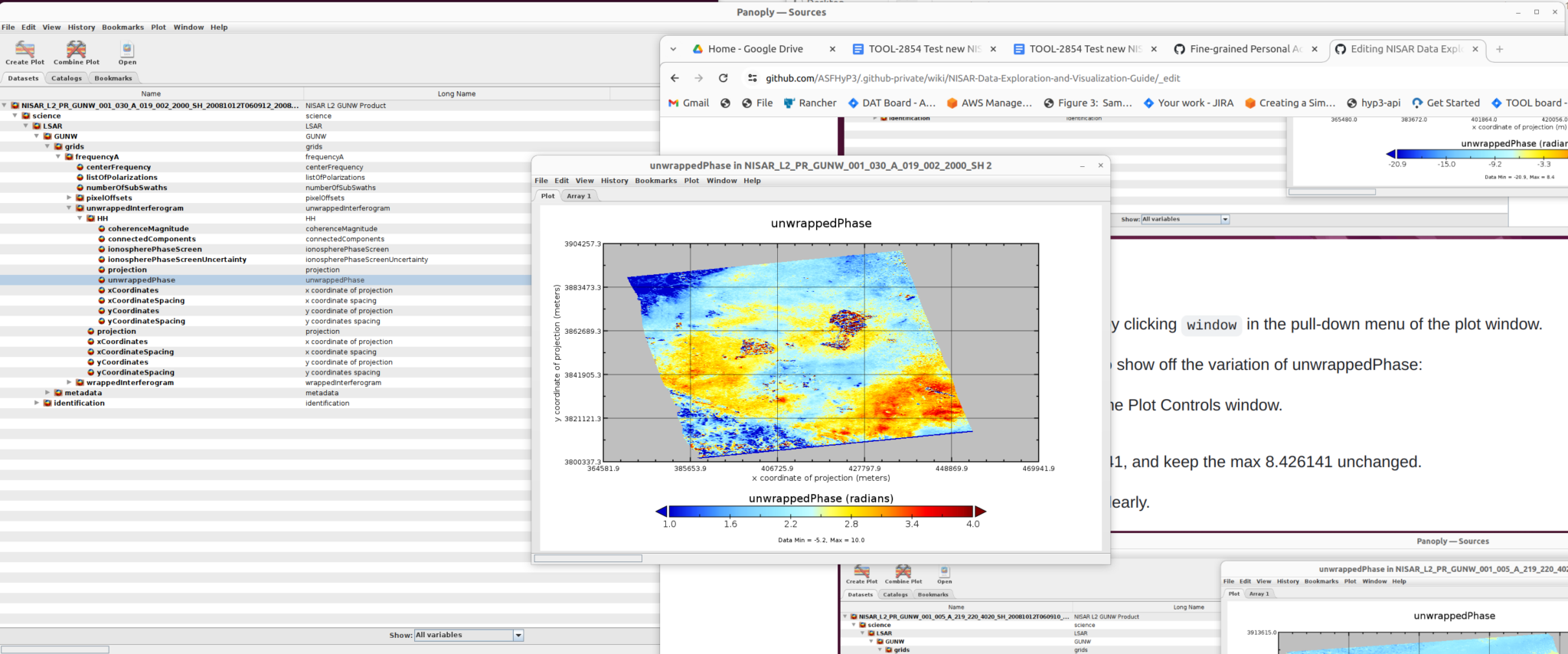
3) Customize the Plot
Users can control the plot properties by clicking window in the pull-down menu of the plot window.
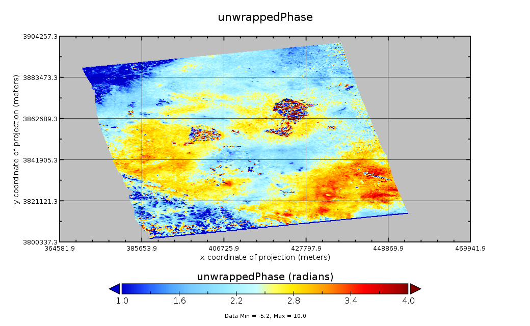
As an example, to change the scale to show off the variation of unwrappedPhase:
- Select
Plot Controlsto open the Plot Controls window - Select
scale - Change the min value to -8.426141, and keep the max 8.426141 unchanged
The new plot displays the variation clearly.
4) Save the Plot
When you are satisfied with the plot, you can save the results.
- Select
Filein the main menu of plot window - Select
Save Imageto open the Save As… window - Select the directory, and either accept the default filename or input the filename of your choice
- Click the
savebutton to save the plot
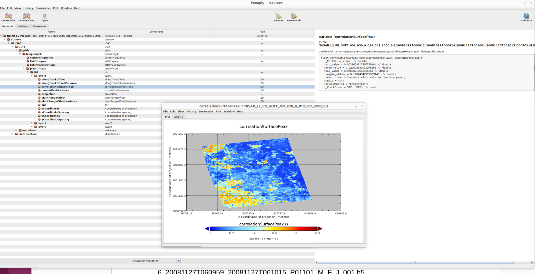
The example GOFF product is:
NISAR_L2_PR_GOFF_001_030_A_019_002_2000_SH_20081012T060912_20081012T060924_20081127T061001_20081127T061013_D00402_M_P_J_001.h5
Use the same process detailed in the GUNW Product section to visualize the GOFF product.
The sample data package includes two GCOV products:
NISAR_L2_PR_GCOV_001_030_A_019_2000_SHNA_A_20081012T060910_20081012T060926_D00402_N_F_J_001.h5
NISAR_L2_PR_GCOV_002_030_A_019_2000_SHNA_A_20081127T060959_20081127T061015_D00402_N_F_J_001.h5
They can be loaded directly in Panoply. Users can explore the data structure of the products and can visualize the 2D variables in the products. We will use the acquisition from 12-Oct-2008 in the illustrations.
For example, we visualize two variables here.
radar_backscatter_gamma0
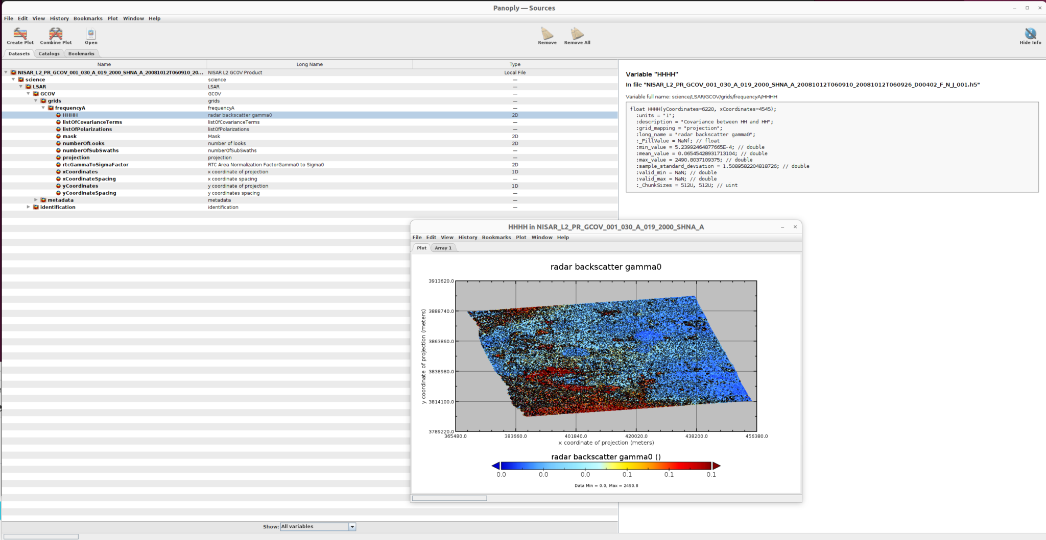
rtcGammaToSigmaFactor
You may need to open the Plot Control window and adjust the grid, scale, and map projection to get a suitable visualization.
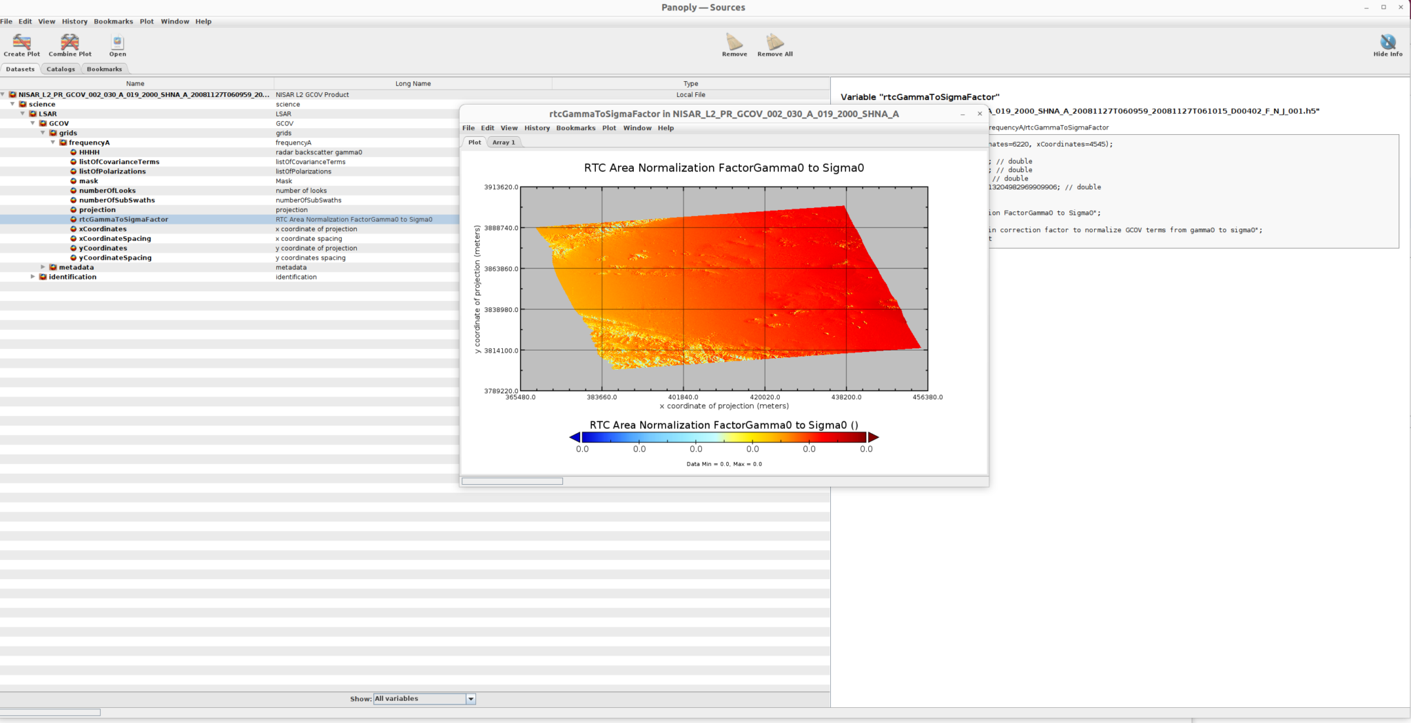
If you choose to create a Georeferenced longitude-latitude color contour plot for a 2D variable, you may need to extract the variable and save it into a NetCDF file, then visualize the NetCDF file. For example, if we want to visualize the rtcGammaToSigmaFactor 2D variable in the file:
gdal_translate -of NetCDF NETCDF:"NISAR_L2_PR_GCOV_001_030_A_019_2000_SHNA_A_20081012T060910_20081012T060926_D00402_N_F_J_001.h5"://science/LSAR/GCOV/grids/frequencyA/rtcGammaToSigmaFactor rtcAreaNormalizationFactorGamma0ToSigma0.nc
Load the NetCDF file into Panoply and plot the variable by choosing the Georeferenced plot type. You may need to open the Plot Control window and adjust the grid, scale, and map projection to get a suitable visualization.
This is the original display of rtcAreaNormalizationFactorGamma0ToSigma0.nc file in Panoply:
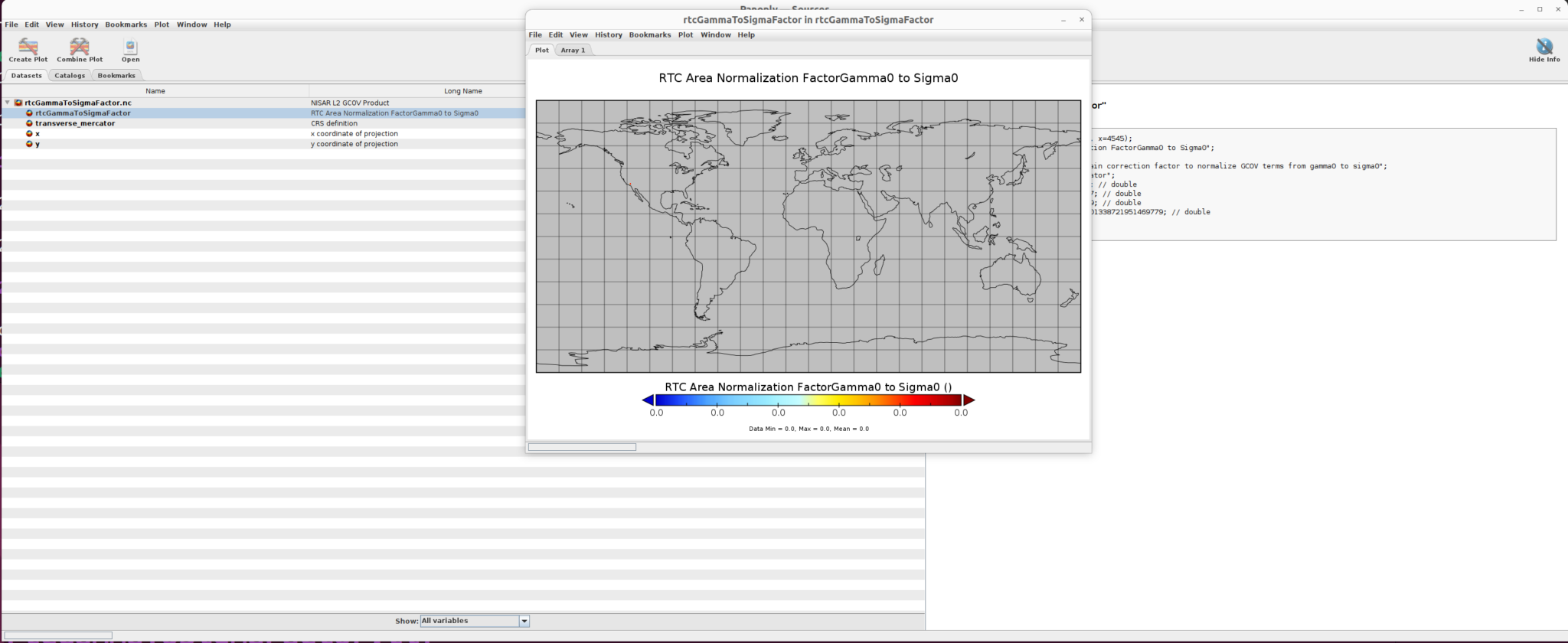
The map projection, scale, and grid adjustments are made in the Plot Control window to visualize the rtcAreaNormalizationFactorGamma0ToSigma0.nc file appropriately:
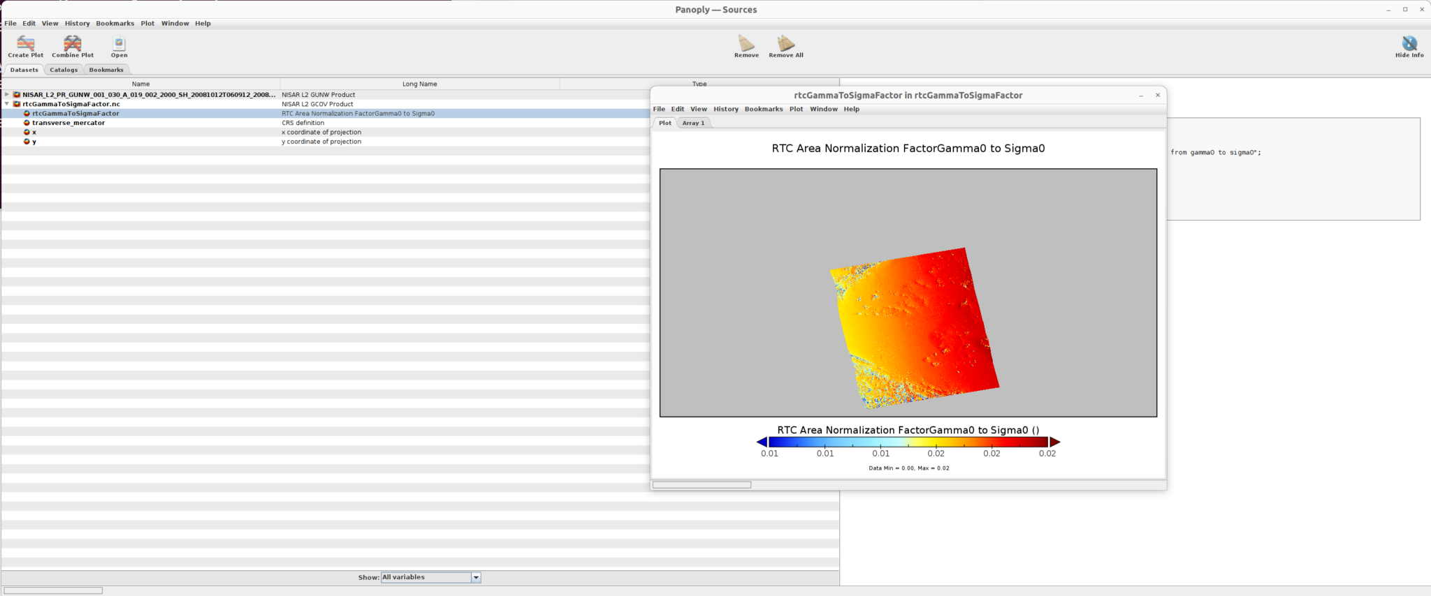
After applying the adjustments, the rtcAreaNormalizationFactorGamma0ToSigma0.nc file is displayed as illustrated below.
There are two GSLC products included in the sample data:
NISAR_L2_PR_GSLC_001_030_A_019_2000_SHNA_A_20081012T060910_20081012T060926_D00402_N_F_J_001.h5
NISAR_L2_PR_GSLC_002_030_A_019_2000_SHNA_A_20081127T060959_20081127T061015_D00402_F_N_J_001.h5
These files can be loaded into Panoply. We will use the acquisition from 12-Oct-2008 in the illustrations.
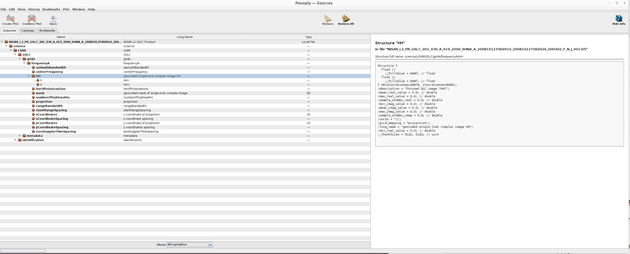
We can explore the datasets in the product. Since the variable HH is complex data, it can not be visualized directly. We can extract the sub-datasets in the h5 file using GDAL, and then visualize these sub-datasets in Panoply.
The subdataset is a complex datatype, so we cannot use the gdal_translate command to convert a complex dataset directly into a NetCDF file. Instead, we use the following logic to generate a file that can be used to visualize the subdataset:
1) Convert the subdataset into a geotiff file
gdal_translate -of GTiff NETCDF:"NISAR_L2_PR_GSLC_001_005_A_219_2005_DHDH_A_20081127T060959_20081127T061015_P01101_N_F_J_001.h5"://science/LSAR/GSLC/grids/frequencyA/HH hh.tif
2) Convert the single-band Complex32 dataset into a two-band Float32 GeoTIFF file
from osgeo import gdal
import numpy as np
gdal.UseExceptions()
file="hh.tif"
outfile = "hh_polar.tif"
ds = gdal.Open(file)
band = ds.GetRasterBand(1)
data = band.ReadAsArray()
amp = abs(data)
phase = np.angle(data)
# create output raster file
driver = gdal.GetDriverByName("GTiff")
outdata = driver.Create(outfile, ds.RasterXSize, ds.RasterYSize, 2, gdal.GDT_Float64)
outdata.SetGeoTransform(ds.GetGeoTransform())
outdata.SetProjection(ds.GetProjection())
outdata.SetMetadata(ds.GetMetadata())
outdata.GetRasterBand(1).WriteArray(amp)
outdata.GetRasterBand(1).SetMetadata({"bandname": "modulus"})
outdata.GetRasterBand(2).WriteArray(phase)
outdata.GetRasterBand(2).SetMetadata({"bandname": "argument"})
outdata = None
3) Convert the GeoTIFF file to a NetCDF file
gdal_translate -of NetCDF hh_polar.tif hh_polar.nc
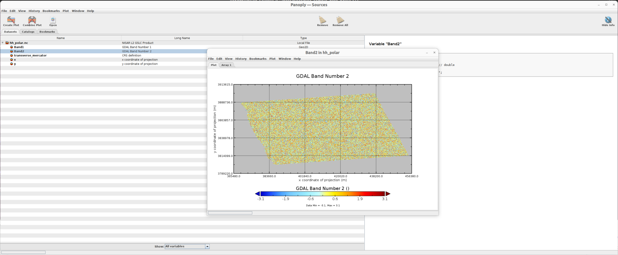
4) Use Panoply to visualize the amplitude and phase data in the NetCDF file
Amplitude data
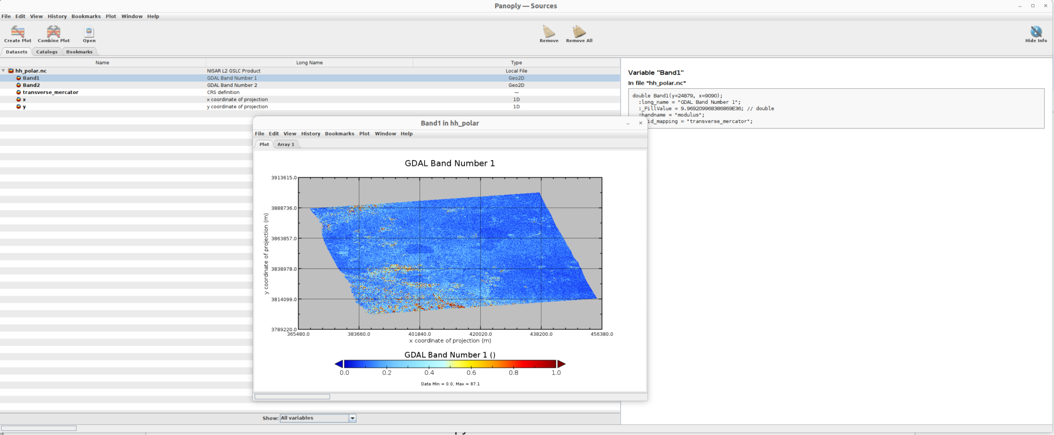
Phase data
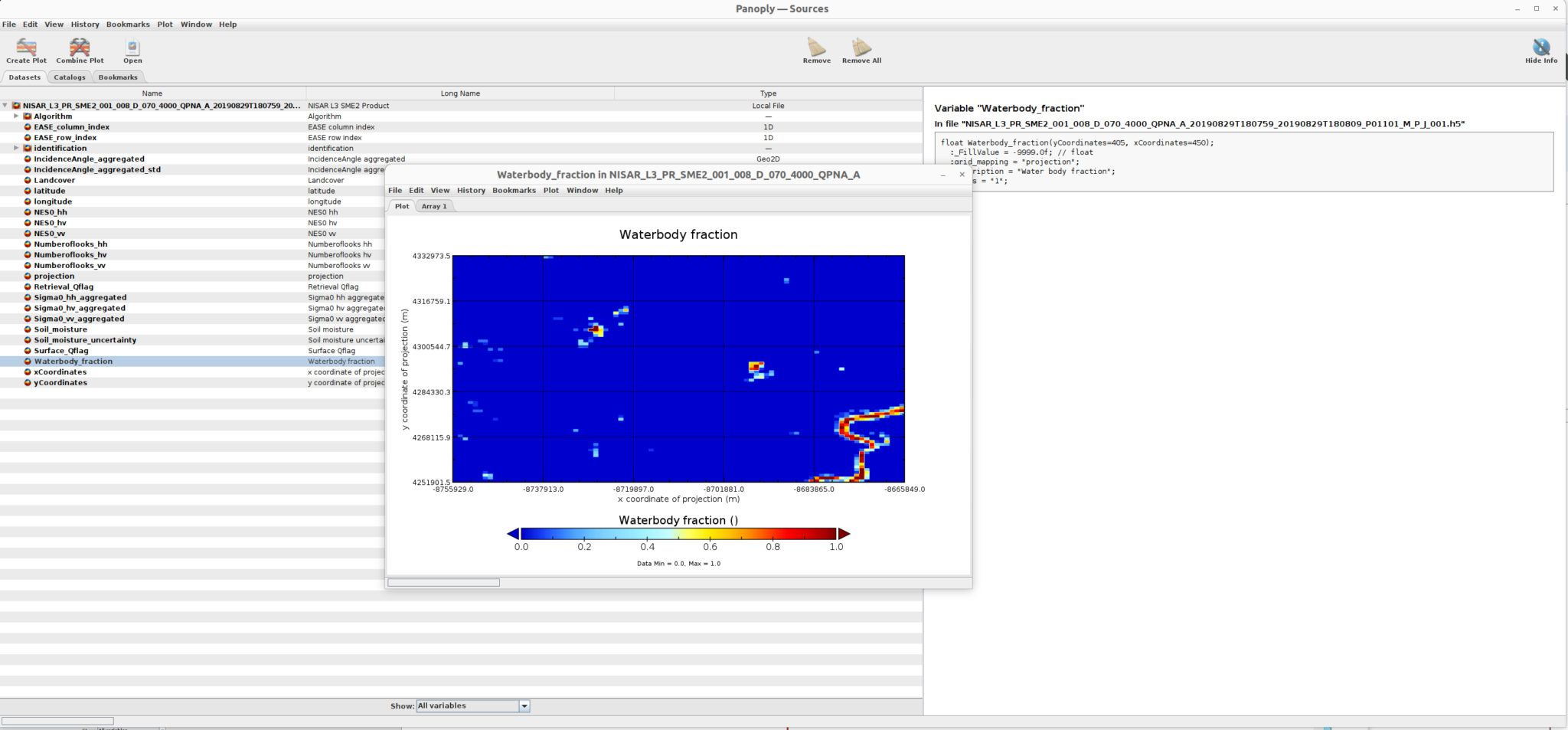
The sample SME2 data is:
NISAR_L3_PR_SME2_001_008_D_070_4000_QPNA_A_20190829T180759_20190829T180809_P01101_M_P_J_001.h5
The SME2 product sub-datasets can be displayed using the same process we used for the GUNW product.
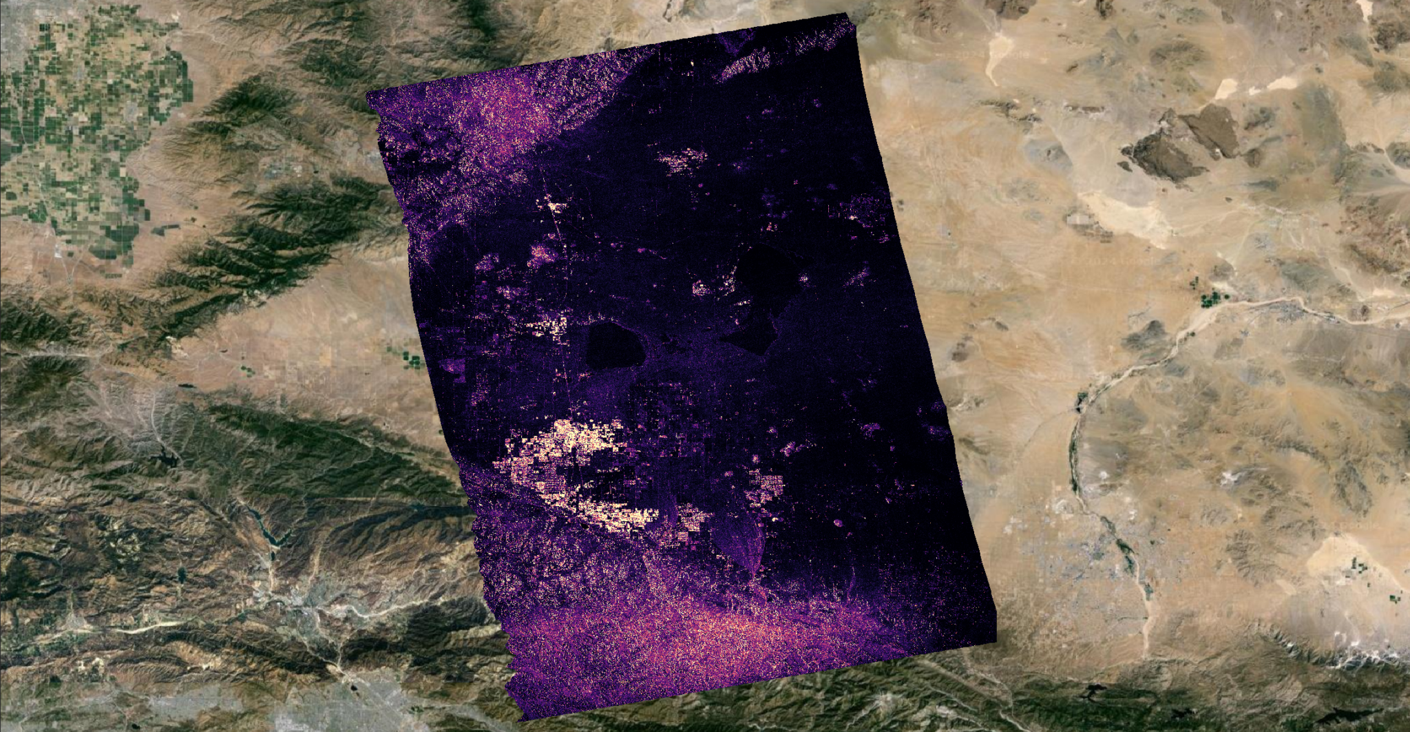
For example, the water body fraction sub-dataset is displayed here:
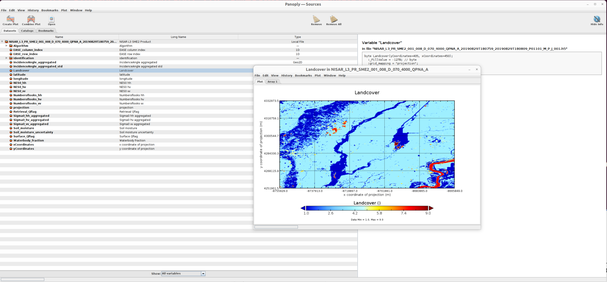
and the landcover sub-dataset is displayed here: